
Humans naturally perceive and interact with the physical world through an interconnected blend of sensory modalities—visual scenes, spoken dialogue, textual symbols, and acoustic signals. Traditional deep learning architectures operated predominantly in isolation, relying on single-modality encoders specialized exclusively for computer vision, natural language processing, or audio signal analysis. In contrast, Multimodal Learning seeks to build unified representations that bridge distinct data modalities within a shared feature space.
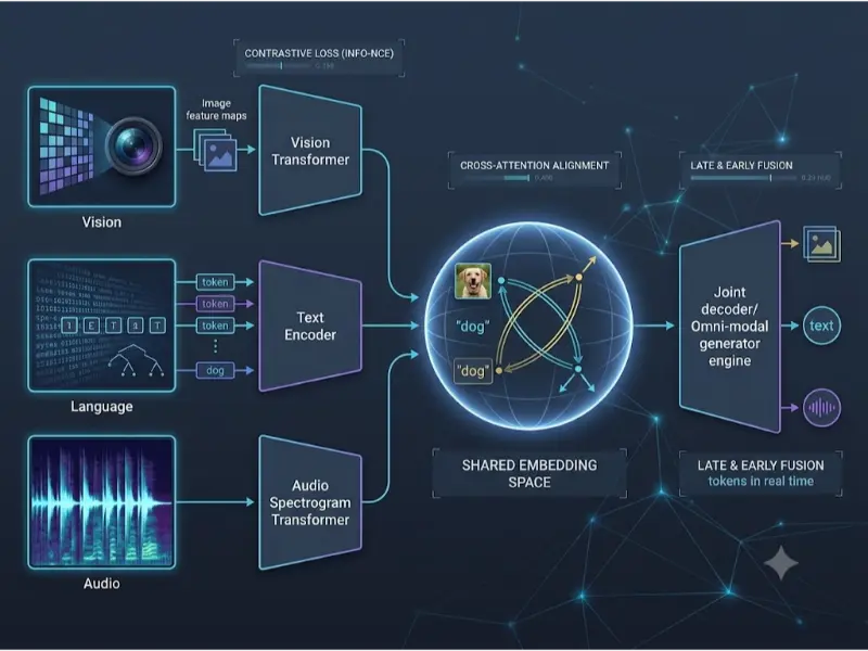
The advancement from early contrastive vision-language models like CLIP (Contrastive Language-Image Pre-training) to modern native, omni-modal foundational systems like GPT-4o represents a major paradigm shift. Rather than relying on late-stage fusion or post-hoc text conversion, contemporary cross-modal architectures align vision, language, and audio streams early in the model topology using cross-attention mechanisms and unified tokenization strategies.
Interactive Quick Review: Early Fusion vs. Late Fusion
What is the primary architectural difference between early-fusion and late-fusion multimodal models, and why is early fusion preferred for native real-time cross-modal interaction?
Toggle Answer
Answer: Late fusion processes each modality independently using separate neural backbone networks and joins their outputs only at the final prediction layer. Early fusion projects distinct visual, audio, and textual inputs into a shared token space early in the model pipeline. This allows cross-attention transformer layers to model fine-grained temporal and spatial dependencies across modalities simultaneously.
Architectural & Theoretical Deep Dives
1. Contrastive Learning Mechanics (CLIP & InfoNCE Loss)
The CLIP architecture aligns visual images and textual descriptions by training an Image Encoder I(·) and a Text Encoder T(·) jointly on a large dataset of (image, text) pairs. Given a mini-batch of N pairs (xiI, xiT), the encoders project inputs into a shared d-dimensional embedding space, yielding normalized feature vectors:
$$v_i = \frac{I(x_i^I)}{\|I(x_i^I)\|_2}, \quad t_i = \frac{T(x_i^T)}{\|T(x_i^T)\|_2}$$
The model calculates a pairwise cosine similarity matrix Si,j = viT tj scaled by a learned temperature parameter τ. The training objective optimizes a symmetric InfoNCE Loss over image-to-text ($L_I$) and text-to-image ($L_T$) classifications:
$$L_I = -\frac{1}{N} \sum_{i=1}^N \log \frac{\exp(v_i^{\text{T}} t_i / \tau)}{\sum_{j=1}^N \exp(v_i^{\text{T}} t_j / \tau)}$$
$$L_T = -\frac{1}{N} \sum_{i=1}^N \log \frac{\exp(t_i^{\text{T}} v_i / \tau)}{\sum_{j=1}^N \exp(t_i^{\text{T}} v_j / \tau)}$$
$$L_{\text{CLIP}} = \frac{1}{2} \left( L_I + L_T \right)$$
2. Cross-Attention Projection & Token Alignment
In autoregressive vision-language models (e.g., LLaVA, Flamingo), visual feature patches extracted from a Vision Transformer (ViT) are mapped into the text decoder’s latent dimension using a trainable linear projection or Perceiver Resampler matrix Wproj:
$$Z_{\text{visual}} = \mathbf{W}_{\text{proj}} \cdot \text{ViT}(X_{\text{image}})$$
The projected visual tokens $Z_{\text{visual}}$ are prepended directly to text token embeddings $Z_{\text{text}}$. Cross-Attention layers update text token representations $H$ by querying visual keys $K_V$ and values $V_V$:
$$\text{Attention}(Q_T, K_V, V_V) = \text{softmax}\left( \frac{Q_T K_V^{\text{T}}}{\sqrt{d_k}} \right) V_V$$
3. Native Omni-Modal Architectures (GPT-4o Style)
Native omni-modal models process audio, visual pixels, and text tokens end-to-end within a single unified Transformer network without routing through separate external ASR (Automatic Speech Recognition) or TTS (Text-to-Speech) engines. Raw audio waveforms are tokenized directly via neural audio codecs (e.g., EnCodec) into discrete acoustic codebook indices. By processing all modalities as an interleaved sequence of tokens, the network achieves low audio-to-audio latency (∼200–300ms) and preserves vocal tone, emotion, and background acoustic context.
4. Python Implementation: Simplified InfoNCE Loss Module
import torch

import torch.nn as nn

import torch.nn.functional as F


class InfoNCELoss(nn.Module):

    """

    Symmetric InfoNCE Loss for cross-modal contrastive embedding alignment.

    """

    def __init__(self, init_temperature: float = 0.07):

        super().__init__()

        self.log_temperature = nn.Parameter(torch.log(torch.tensor(init_temperature)))


    def forward(self, image_features: torch.Tensor, text_features: torch.Tensor):

        # L2 Normalize embeddings along feature dimension

        img_norm = F.normalize(image_features, p=2, dim=-1)

        txt_norm = F.normalize(text_features, p=2, dim=-1)


        # Compute scaled cosine similarity matrix (N x N)

        temp = torch.exp(self.log_temperature)

        logits = torch.matmul(img_norm, txt_norm.T) / temp


        # Labels are diagonal indices (matching image-text pairs)

        labels = torch.arange(logits.shape[0], device=logits.device)


        loss_img = F.cross_entropy(logits, labels)

        loss_txt = F.cross_entropy(logits.T, labels)


        return (loss_img + loss_txt) / 2.0


# Example Usage: Batch of 4 items with 512-dimensional embeddings

img_emb = torch.randn(4, 512)

txt_emb = torch.randn(4, 512)

loss_fn = InfoNCELoss()

loss_val = loss_fn(img_emb, txt_emb)

print("InfoNCE Batch Loss:", loss_val.item())
Interactive Quick Review: Zero-Shot Classification Mechanics
How does a trained CLIP model perform zero-shot visual classification without fine-tuning on a target dataset?
Toggle Answer
Answer: Target class names are converted into text prompts (e.g., “a photo of a [label]”) and passed through the Text Encoder to create a bank of normalized class embeddings. An input image is passed through the Image Encoder to produce an image embedding. The predicted class is selected by computing the highest cosine similarity between the image embedding and the prompt embeddings.
Taxonomy & Optimization Comparison Matrix
| Architecture Style | Supported Modalities | Fusion Point | Inference Overhead | Primary Advantage |
|---|---|---|---|---|
| Contrastive Dual-Encoder (e.g., CLIP) | Vision + Text | Late Shared Projection Space | Low (Independent Encoders) | Zero-shot cross-modal retrieval & indexing |
| Cross-Attention Adapter (e.g., Flamingo) | Vision + Interleaved Text | Mid-Fusion via Gated Cross-Attention | Moderate | In-context visual reasoning and captioning |
| Linear Projection VLM (e.g., LLaVA) | Vision + Text | Early Token Mapping to LLM | High (Full LLM execution) | Detailed visual QA and conversational logic |
| Native Omni-Modal (e.g., GPT-4o) | Vision + Language + Audio | Early Unified Token Stream | High (End-to-End Processing) | Ultra-low audio latency & emotion preservation |
Applications, Trade-offs, & Future Outlook
Real-World Applications
- Real-Time Conversational Assistants: Sub-second voice-to-voice interaction handling interruptions, vocal inflections, and live visual inputs simultaneously.
- Autonomous Robotics: Embodied visual-language-action (VLA) models mapping visual camera feeds and natural language commands directly to robotic motor control tokens.
- Medical Diagnostics: Joint alignment of radiographic scans (DICOM), clinical notes, and physician dictations for comprehensive diagnostic reporting.
Engineering Trade-offs
Aligning heterogeneous data modalities introduces severe compute and data challenges. High-resolution vision tokens (e.g., 256 tokens per frame) rapidly expand transformer context windows, dramatically increasing quadratic self-attention memory overhead ($O(N^2)$). Furthermore, balancing loss weights across modalities during pre-training often leads to “modality dominance,” where the model favors dominant text signals over subtle audio or visual cues.
Future Outlook & Emerging Research
Next-generation multimodal research focuses on Sub-Quadratic Context Scaling (utilizing State Space Models like Mamba alongside linear attention) to process long-form multi-hour video streams. Concurrently, native continuous tokenizers are being developed to bypass discrete codebook bottleneck quantization errors entirely.
Frequently Asked Questions
What is Modality Collapse in multimodal learning?
Modality collapse occurs during joint pre-training when the cross-modal projection layer maps vastly different visual or audio inputs to a narrow, uninformative cluster in the shared latent space, preventing effective cross-modal distinction.
Why is a learned temperature parameter τ necessary in contrastive loss?
The temperature parameter τ scales the magnitudes of cosine similarities prior to the softmax calculation. A trainable τ prevents gradients from vanishing or exploding as embeddings normalize, ensuring the model scales logit sensitivity dynamically during training.
How do visual tokenizers compress high-resolution image inputs?
Visual encoders like ViT divide an image into non-overlapping spatial patches (e.g., 14×14 pixels) and linearly project each patch into an embedding vector. Advanced architectures utilize visual resamplers or Q-Formers to downsample hundreds of patch embeddings into a fixed set of (e.g., 32 or 64) salient visual tokens.
What is the benefit of processing raw audio codecs directly instead of spectrograms?
While mel-spectrograms capture frequency-domain energy over time, they lose fine phase details and increase latency due to STFT windowing delays. Discrete neural audio codecs (like EnCodec or SoundStream) encode raw waveform audio into ultra-compact, streamable discrete tokens suitable for real-time bidirectional synthesis.
End-of-Page Exercises & Assessment
Part 1: Review Questions
Q1: Define the InfoNCE loss function used in CLIP pre-training.
Answer: InfoNCE is a categorical cross-entropy loss applied over normalized cosine similarity scores across paired positive cross-modal samples against all negative batch samples, driving positive image-text pairs together while repelling un-matched pairs in latent space.
Q2: What role does a Projection Head (e.g., Wproj) play in Vision-Language Models?
Answer: The projection head maps output feature vectors from a visual encoder (e.g., ViT output dimension 1024) into the exact hidden dimension space expected by the language model (e.g., LLM text token dimension 4096).
Q3: Explain how Zero-Shot Prompting works in visual classification.
Answer: Zero-shot prompting replaces fixed one-hot class outputs by mapping class labels into natural text templates, encoding them via a text transformer, and measuring cosine similarity against input image embeddings.
Q4: What causes quadratic complexity growth when ingesting video in Multimodal Transformers?
Answer: Full self-attention calculates dot-product attention scores across every pair of sequence tokens. Ingesting multiple video frames produces thousands of visual patch tokens, causing memory and compute requirements to scale quadratically with sequence length ($O(N^2)$).
Q5: State the primary advantage of native omni-modal models over multi-stage cascaded systems.
Answer: Native omni-modal models eliminate serial pipeline latency (speech-to-text -> LLM -> text-to-speech) and retain non-verbal acoustic signals (emotion, tone, pitch, background noise) that are lost when converting speech to intermediate text.
Part 2: Thought-Provoking Questions
Q1: Modality Bias and Hallucination Mechanics
Scenario: A Vision-Language Model is presented with an image of an empty dining table alongside the text prompt: “List the fruits in the bowl on the table.” The model hallucinates an detailed list of apples and bananas even though no bowl exists.
Analysis: Hallucination occurs because the auto-regressive language prior in the decoder overpowers weak cross-attention signals from visual tokens (“modality dominance”). When text prompts contain strong contextual priors, the language backbone predicts highly probable word continuations regardless of visual patch token constraints. Mitigating this requires balanced multimodal instruction tuning and contrastive decoding.
Q2: Privacy & Real-time Edge Streaming
Scenario: Compare the architectural trade-offs of running an omni-modal vision-audio model locally on smart glasses vs. offloading visual/audio streams to a cloud server over 5G.
Analysis: Local edge deployment eliminates network transmission latency, operates offline, and ensures maximum user privacy (raw video/audio streams never leave the device), but requires extreme quantization (INT4) and small parameter scales (1B–3B parameters). Cloud offloading permits high-capacity models (70B+ parameters) with superior reasoning capabilities but introduces non-deterministic network latency (100–500ms) and privacy compliance risks.
Part 3: Numerical Engineering Problems
Problem 1: Pairwise Cosine Similarity & InfoNCE Logit Calculation
Question: Given an image embedding vector $v = [0.6, \; 0.8]$ and a text embedding vector $t = [0.8, \; 0.6]$, both already normalized to unit length ($\|v\|_2 = \|t\|_2 = 1$). Assuming a temperature parameter $\tau = 0.05$, calculate:
1. The raw cosine similarity $S = v^{\text{T}} t$.
2. The scaled logit value $L = \frac{v^{\text{T}} t}{\tau}$ used in the softmax denominator.
Step-by-step Solution:
1. Calculate dot product (cosine similarity): $$S = v^{\text{T}} t = (0.6 \times 0.8) + (0.8 \times 0.6) = 0.48 + 0.48 = 0.96$$
2. Apply temperature scaling ($\tau = 0.05$): $$L = \frac{S}{\tau} = \frac{0.96}{0.05} = 19.2$$
Final Answer: Cosine similarity $S = \mathbf{0.96}$, and the scaled logit value is $\mathbf{19.2}$.
Problem 2: Visual Patch Token Count Calculation
Question: An input image with resolution $H = 448$ pixels and $W = 448$ pixels is processed by a Vision Transformer using non-overlapping patches of size $P = 14 \times 14$ pixels.
1. Calculate the total number of visual patch tokens $N_{\text{patches}}$ generated by the encoder.
2. If each patch token has hidden dimension $D = 1024$ in FP16 precision (2 bytes per element), calculate the memory size in megabytes (MB) required to store this single image’s visual token tensor.
Step-by-step Solution:
1. Calculate the number of visual patches: $$N_{\text{patches}} = \left( \frac{H}{P} \right) \times \left( \frac{W}{P} \right) = \left( \frac{448}{14} \right) \times \left( \frac{448}{14} \right) = 32 \times 32 = 1024 \text{ tokens}$$
2. Calculate total tensor memory size in bytes: $$\text{Total Elements} = N_{\text{patches}} \times D = 1024 \times 1024 = 1,048,576 \text{ elements}$$ $$\text{Memory Bytes} = 1,048,576 \times 2 \text{ bytes} = 2,097,152 \text{ bytes}$$ $$\text{Memory MB} = \frac{2,097,152}{10^6} \approx 2.097 \text{ MB} \quad (\text{or } \frac{2,097,152}{1,048,576} = 2.00 \text{ MiB})$$
Final Answer: The image produces $\mathbf{1024 \text{ tokens}}$, requiring exactly $\mathbf{2.00 \text{ MiB}}$ ($2.097 \text{ MB}$) of RAM.
Advanced Neural Architectures Sub-Cluster
-
Diffusion Models & GANs
Explore Stable Diffusion, score-based generative architectures, and latent space diffusion mechanics. -
Efficient Deep Learning & Quantization
Master model compression, INT8/FP4 quantization, channel pruning, and edge acceleration. -
NAS & AutoML
Learn automated hyperparameter tuning, neural topology optimization, and zero-cost proxies.
External Academic & Technical References
- Learning Transferable Visual Models From Natural Language Supervision (Radford et al., OpenAI CLIP) – Seminal paper establishing contrastive vision-language representation learning.
- Visual Instruction Tuning (Liu et al., LLaVA) – Foundational open-source architecture for visual instruction tuning using linear projection layers.
- GPT-4o System Architecture & Capabilities Overview – Technical deep dive into native omni-modal processing across vision, text, and voice modalities.