
Generative modeling represents one of the most mathematically profound frontiers in modern artificial intelligence. Unlike discriminative models that learn conditional probability distributions P(Y | X) to predict target labels from inputs, generative frameworks model the underlying data distribution P(X) directly. This enables the synthesis of novel, high-dimensional data samples—such as photo-realistic images, complex audio waveforms, and molecular structures—that are statistically indistinguishable from real training data.
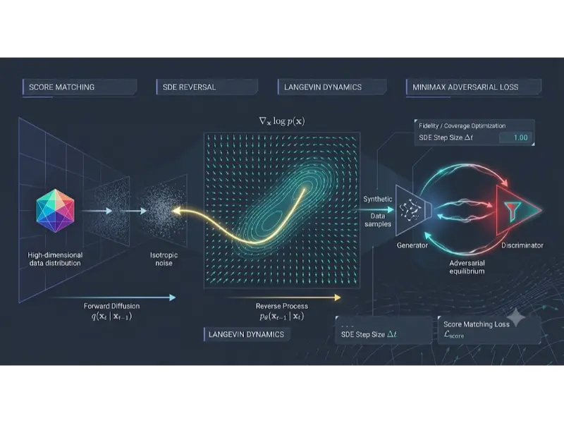
The evolution of deep generative models spans three major paradigm families: Generative Adversarial Networks (GANs), which optimize a two-player minimax game; Score-Based Generative Models, which estimate the gradient of the log probability density using score matching; and Denoising Diffusion Probabilistic Models (DDPMs), which model generation as a gradual reverse Markovian denoising process. Understanding these mechanics provides the structural foundation for state-of-the-art architectures like Stable Diffusion and latent diffusion pipelines.
Interactive Quick Review: Mode Collapse vs. Training Stability
Why do Denoising Diffusion Probabilistic Models (DDPMs) exhibit superior training stability and sample coverage compared to Generative Adversarial Networks (GANs)?
Toggle Answer
Answer: GANs rely on a delicate adversarial minimax equilibrium between a generator and discriminator, making them highly susceptible to mode collapse and vanishing gradients. In contrast, diffusion models are trained using a stable, maximum-likelihood-surrogate objective (evidence lower bound / score matching loss) that optimizes a sequence of well-behaved denoising autoencoders across fixed timestep scales.
Architectural & Theoretical Deep Dives
1. Denoising Diffusion Probabilistic Models (DDPM) Mechanics
Diffusion models define a two-phase Markovian process: a Forward Diffusion Process that systematically destroys structure by adding Gaussian noise, and a Reverse Process that learns to recover original data from pure noise.
Given an initial data distribution x0 ∼ q(x), the forward Markov process adds Gaussian noise across discrete timesteps t = 1, …, T according to a variance schedule β1, …, βT:
$$q(x_t | x_{t-1}) = \mathcal{N}\left(x_t; \; \sqrt{1 – \beta_t} \, x_{t-1}, \; \beta_t \mathbf{I}\right)$$
Using the notation αt = 1 – βt and ᾱt = ∏s=1t αs, we can sample xt directly at any arbitrary timestep t in closed form without iterating:
$$x_t = \sqrt{\bar{\alpha}_t} \, x_0 + \sqrt{1 – \bar{\alpha}_t} \, \epsilon, \quad \epsilon \sim \mathcal{N}(\mathbf{0}, \mathbf{I})$$
The neural network εθ(xt, t) is trained to predict the added Gaussian noise vector ε by minimizing the simplified mean squared error objective:
$$L_{\text{simple}}(\theta) = \mathbb{E}_{t, x_0, \epsilon} \left[ \left\| \epsilon – \epsilon_\theta\left( \sqrt{\bar{\alpha}_t} x_0 + \sqrt{1 – \bar{\alpha}_t} \epsilon, \; t \right) \right\|^2 \right]$$
2. Score-Based Generative Models & Continuous SDE Formulation
Score-based generative models unify discrete diffusion processes through the lens of continuous-time Stochastic Differential Equations (SDEs). Rather than predicting discrete noise vectors, the network learns the Stein Score Function, defined as the gradient of the log probability density with respect to the data:
$$s_\theta(x, t) \approx \nabla_x \log p_t(x)$$
As demonstrated by Song et al., the forward noise corruption can be formulated as an Itô SDE:
$$dx = f(x, t) dt + g(t) d w$$
Remarkably, Anderson’s reverse-time theorem proves that the reverse generative trajectory follows a corresponding reverse-time SDE solved backward in time from t = T to t = 0:
$$dx = \left[ f(x, t) – g(t)^2 \nabla_x \log p_t(x) \right] dt + g(t) d \bar{w}$$
3. Generative Adversarial Networks (GANs) Mechanics
Generative Adversarial Networks formulate sample generation as a zero-sum game between two competing neural architectures: a Generator Gθ(z) that maps random latent noise vectors z ∼ pz(z) to synthetic data samples, and a Discriminator Dφ(x) that outputs the probability that a given sample x originated from the real training set rather than the generator.
The objective function is expressed as the classic Minimax Value Function V(D, G):
$$\min_G \max_D V(D, G) = \mathbb{E}_{x \sim p_{\text{data}}(x)} \left[ \log D(x) \right] + \mathbb{E}_{z \sim p_z(z)} \left[ \log \left(1 – D(G(z))\right) \right]$$
4. Python Implementation: Basic DDPM Forward Noise Sampling Routine
import torch

import torch.nn as nn


def extract_at_indices(values: torch.Tensor, t: torch.Tensor, x_shape: torch.Size):

    """

    Extracts specific broadcastable tensor values at requested batch timesteps.

    """

    batch_size = t.shape[0]

    out = values.gather(-1, t)

    return out.reshape(batch_size, *((1,) * (len(x_shape) - 1)))


def q_sample_forward(x_0: torch.Tensor, t: torch.Tensor, alpha_cumprod: torch.Tensor):

    """

    Samples x_t in closed form given x_0, timestep t, and precalculated alpha_cumprod values.

    """

    noise = torch.randn_like(x_0)

    sqrt_alpha_cumprod = torch.sqrt(extract_at_indices(alpha_cumprod, t, x_0.shape))

    sqrt_one_minus_alpha_cumprod = torch.sqrt(1.0 - extract_at_indices(alpha_cumprod, t, x_0.shape))


    x_t = sqrt_alpha_cumprod * x_0 + sqrt_one_minus_alpha_cumprod * noise

    return x_t, noise


# Example setup for 1000 diffusion steps

timesteps = 1000

beta_schedule = torch.linspace(1e-4, 0.02, timesteps)

alpha_schedule = 1.0 - beta_schedule

alpha_cumprod = torch.cumprod(alpha_schedule, dim=0)


# Batch of 4 dummy image tensors (Channels=3, H=32, W=32)

x_0_batch = torch.randn(4, 3, 32, 32)

t_batch = torch.tensor([10, 250, 500, 999], dtype=torch.long)


x_t_noisy, noise_target = q_sample_forward(x_0_batch, t_batch, alpha_cumprod)

print("Noisy Tensor Shape:", x_t_noisy.shape)

print("Target Noise Shape:", noise_target.shape)
Interactive Quick Review: Score Functions & Normalizing Constants
Why is calculating the Stein Score Function ∇x log p(x) computationally advantageous over evaluating the raw probability density function p(x)?
Toggle Answer
Answer: Any unnormalized probability distribution can be written as p(x) = p̃(x) / Z, where Z is the intractable partition function (normalizing constant). Taking the gradient of the log density cancels out Z entirely (∇x log p(x) = ∇x log p̃(x) – ∇x log Z = ∇x log p̃(x)), bypassing the need to compute high-dimensional integrals.
Taxonomy & Optimization Comparison Matrix
| Model Paradigm | Inference Speed | Sample Quality | Mode Coverage (Diversity) | Mathematical Training Loss |
|---|---|---|---|---|
| DDPM / DDIM | Slow (Iterative 50–1000 steps) | State-of-the-Art (High) | High (No mode collapse) | MSE Noise Prediction Error (ELBO surrogate) |
| Score-Based SDEs | Variable (Numerical SDE/ODE solvers) | State-of-the-Art (High) | High (Exact density recovery) | Denoising Score Matching Loss |
| Generative Adversarial Networks | Fast (Single Forward Pass) | Very High (Sharp textures) | Prone to Mode Collapse | Adversarial Minimax Loss / Wasserstein Loss |
| Latent Diffusion (e.g., LDM) | Moderate (5–50 steps in compressed space) | State-of-the-Art (High) | High | Latent Space Perceptual Noise Loss |
| Flow Matching / Consistency Models | Ultra-Fast (1–4 sampling steps) | High | High | Vector Field Regression Loss |
Applications, Trade-offs, & Future Outlook
Real-World Applications
- Text-to-Image & Video Generation: Foundation models (Stable Diffusion, Midjourney, Sora) leveraging latent diffusion and classifier-free guidance for controllable content creation.
- Structural Biology & Drug Discovery: Utilizing score-based generative 3D point cloud architectures to generate valid novel molecular structures and protein binders.
- Medical Image Restoration: Super-resolution, artifact removal, and low-dose MRI/CT reconstruction via conditional diffusion reverse sampling.
Engineering Trade-offs
While diffusion models offer unmatched sample fidelity and complete mode distribution coverage, their multi-step iterative nature presents severe inference latency overhead compared to single-pass GAN generators. Accelerating inference requires advanced techniques like Probability Flow ODE distillations, Classifier-Free Guidance (CFG) tuning, or transitioning directly to latent-space execution.
Future Outlook & Emerging Research
The field is rapidly converging toward Rectified Flow Matching and Consistency Models, which map Gaussian noise straight to target data distributions via straight linear trajectories. This allows continuous score-based models to generate high-fidelity samples in as few as 1 to 4 inference steps while preserving strict probabilistic rigor.
Frequently Asked Questions
What is the difference between DDPM and DDIM?
DDPM (Denoising Diffusion Probabilistic Models) uses a stochastic Markovian reverse process requiring hundreds of steps. DDIM (Denoising Diffusion Implicit Models) generalizes DDPM to a non-Markovian deterministic process governed by a Probability Flow ODE. This allows DDIM to skip timesteps during sampling, reducing required inference steps by 10× to 50× without retraining.
How does Classifier-Free Guidance (CFG) work in text-to-image diffusion?
CFG jointly trains a single diffusion network on conditioned inputs (e.g., text prompt) and unconditioned inputs (e.g., null prompt). During reverse sampling, the predicted noise is extrapolated away from the unconditioned estimate toward the conditioned estimate using a scalar weight w: ε̂ = εuncond + w(εcond – εuncond), significantly improving prompt alignment.
Why are Latent Diffusion Models (LDMs) more efficient than Pixel-Space Diffusion Models?
Pixel-space models run expensive U-Net convolutions at high spatial resolution (e.g., 512×512 px). LDMs first compress images into a perceptually equivalent, low-dimensional latent space (e.g., 64×64 px) using a pre-trained Autoencoder (VAE), performing the reverse diffusion steps in this compact space to drastically lower computational compute.
What causes mode collapse in GANs?
Mode collapse occurs when the generator finds a narrow subset of outputs that successfully fools the discriminator, causing it to repeatedly produce identical samples regardless of latent noise variations. This stems from instabilities in solving the non-convex minimax game using gradient descent.
End-of-Page Exercises & Assessment
Part 1: Review Questions
Q1: Define the forward process in a Denoising Diffusion Probabilistic Model (DDPM).
Answer: The forward process is a fixed, non-learnable Markov chain that gradually converts a clean data sample x0 into isotropic Gaussian noise xT over T timesteps by adding small amounts of Gaussian noise governed by a variance schedule βt.
Q2: State the Minimax loss function of a standard Generative Adversarial Network (GAN).
Answer: minG maxD V(D, G) = &mathbb;Ex∼pdata[log D(x)] + &mathbb;Ez∼pz[log(1 – D(G(z)))].
Q3: What is the Stein Score Function?
Answer: The Stein Score Function is the spatial gradient vector field of the log probability density with respect to the input variable x, formally written as ∇x log p(x).
Q4: What key advantage does a Probability Flow ODE offer over SDE-based reverse diffusion sampling?
Answer: A Probability Flow ODE defines a continuous deterministic trajectory with the same marginal probability densities as the reverse SDE. Because it is deterministic, it enables bidirectional latent space encoding/inversion and fast adaptive ODE numerical integration.
Q5: Explain how the Straight-Through Estimator or Variational Lower Bound (ELBO) relates to DDPM loss.
Answer: The DDPM training objective is mathematically derived from the Variational Lower Bound (ELBO) on the negative log-likelihood -log pθ(x0). Optimizing the simplified noise prediction loss Lsimple acts as a weighted surrogate that maximizes the ELBO.
Part 2: Thought-Provoking Questions
Q1: Trade-offs in High-Throughput Production Systems
Scenario: An enterprise media platform needs to generate 100,000 personalized visual assets per second with strict latency limits (< 50ms per item). Compare the system deployment challenges of using an optimized StyleGAN3 pipeline vs. a 50-step Latent Diffusion Model.
Analysis: StyleGAN3 generates outputs in a single forward pass (< 10ms on modern GPUs), easily achieving high throughput with minimal compute infrastructure. Conversely, a 50-step LDM requires 50 sequential forward passes through a heavy U-Net model, resulting in latencies of 500ms–2000ms. For ultra-high throughput under 50ms, StyleGAN3 or a distilled single-step Consistency/Flow Model is required.
Q2: Deterministic Latent Inversion and Image Editing
Scenario: Why is exact image inversion (mapping a real photo to its precise latent representation) inherently difficult in stochastic DDPMs, and how do deterministic DDIMs resolve this challenge?
Analysis: Stochastic DDPMs inject random Gaussian noise at every reverse sampling step, creating non-deterministic, branching generation paths that make exact reverse trajectory tracing impossible. DDIM removes stochastic noise terms from the reverse step, converting sampling into a deterministic ODE trajectory. Reversing the step direction in DDIM traces the exact same continuous path backward, encoding real images into latent space flawlessly for downstream attribute editing.
Part 3: Numerical Engineering Problems
Problem 1: Direct Forward Closed-Form Diffusion Sampling
Question: Given an original 1D data point x0 = 4.0, a variance schedule step βt = 0.05, and cumulative parameter ᾱt = 0.64 at timestep t = 100, calculate the noisy sample x100 when the sampled Gaussian noise value is ε = -0.5.
Step-by-step Solution:
1. Identify the closed-form forward sampling equation: $$x_t = \sqrt{\bar{\alpha}_t} \, x_0 + \sqrt{1 – \bar{\alpha}_t} \, \epsilon$$
2. Calculate the square root coefficients for ᾱ100 = 0.64: $$\sqrt{\bar{\alpha}_{100}} = \sqrt{0.64} = 0.8$$ $$\sqrt{1 – \bar{\alpha}_{100}} = \sqrt{1 – 0.64} = \sqrt{0.36} = 0.6$$
3. Substitute values into the equation (x0 = 4.0, ε = -0.5): $$x_{100} = (0.8 \times 4.0) + (0.6 \times -0.5)$$ $$x_{100} = 3.2 – 0.3 = 2.9$$
Final Answer: The exact noisy sample value at timestep t = 100 is 2.9.
Problem 2: Discriminator Binary Cross-Entropy Loss Calculation
Question: In a GAN training step, a Discriminator D evaluates 2 real samples and 2 synthetic samples from Generator G. The output probabilities are:
• Real samples: D(x1) = 0.9, D(x2) = 0.8
• Fake samples: D(G(z1)) = 0.3, D(G(z2)) = 0.4
Calculate the total binary cross-entropy loss LD for the Discriminator over this mini-batch.
Step-by-step Solution:
1. State the Discriminator Binary Cross-Entropy loss formula: $$L_D = -\frac{1}{N} \sum_{i=1}^N \left[ \log D(x_i) + \log(1 – D(G(z_i))) \right]$$
2. Evaluate individual log probability terms (using natural log ln):
• Real 1: ln(0.9) ≈ -0.1054
• Real 2: ln(0.8) ≈ -0.2231
• Fake 1: ln(1 – 0.3) = ln(0.7) ≈ -0.3567
• Fake 2: ln(1 – 0.4) = ln(0.6) ≈ -0.5108
3. Sum terms and divide by batch count N = 2 paired observations: $$\text{Sum} = (-0.1054) + (-0.2231) + (-0.3567) + (-0.5108) = -1.1960$$ $$L_D = -\frac{1}{2} (-1.1960) = 0.5980$$
Final Answer: The Discriminator mini-batch loss LD is approximately 0.598.
Advanced Neural Architectures Sub-Cluster
-
Efficient Deep Learning & Quantization
Master model compression, INT8/FP4 quantization, channel pruning, and edge acceleration. -
Multimodal Learning
Dive into joint vision-language-audio representations, CLIP contrastive learning, and GPT-4o style systems. -
NAS & AutoML
Learn automated hyperparameter tuning, neural topology optimization, and zero-cost proxies.
External Academic & Technical References
- Denoising Diffusion Probabilistic Models (Ho et al., 2020) – The seminal paper establishing modern DDPM mechanics and simplified noise loss.
- Score-Based Generative Modeling through Stochastic Differential Equations (Song et al., ICLR 2021) – The theoretical unifying continuous SDE framework for score-based models.
- High-Resolution Image Synthesis with Latent Diffusion Models (Rombach et al., CVPR 2022) – The official research foundation behind Stable Diffusion.