
Modern state-of-the-art neural architectures frequently contain tens to hundreds of billions of parameters. While these massive models demonstrate remarkable generalization and contextual reasoning capabilities, their memory footprint and computational requirements create severe bottlenecks during real-world inference. Deploying large models on edge platforms—such as smartphones, autonomous vehicles, industrial IoT devices, and embedded robotics—demands strict latency bounds, ultra-low energy consumption, and highly efficient memory throughput.
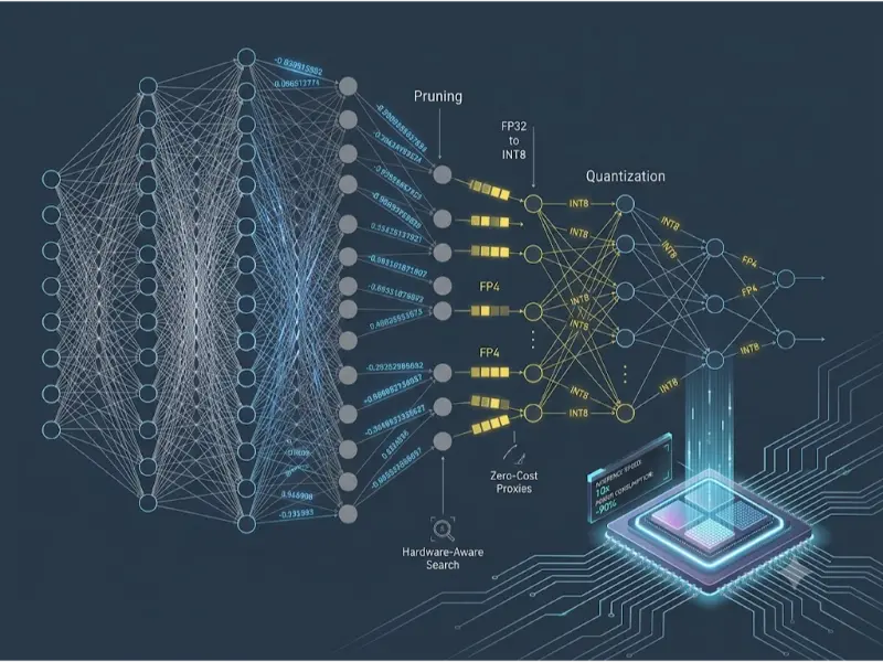
Efficient Deep Learning encompasses a cohesive set of techniques designed to reduce compute cost (FLOPs), reduce dynamic RAM memory bandwidth bottlenecks, and accelerate execution latency without causing unacceptable drops in model accuracy. The three primary pillars of model compression include Quantization, Neural Pruning, and Knowledge Distillation, coupled with hardware-aware optimization compilers targeting Edge Accelerators (NPUs, TPUs, and GPUs).
Interactive Quick Review: Compute vs. Memory Bandwidth Limits
Why is memory bandwidth often a bigger bottleneck than raw computational compute (FLOPs) during single-batch edge neural network inference?
Toggle Answer
Answer: During single-batch inference (batch size = 1), matrix multiplications are bandwidth-bound rather than compute-bound. The system spends significantly more time and energy transferring high-precision model weights from external DRAM into local SRAM cache than it spends performing the actual mathematical multiply-accumulate (MAC) operations. Quantization reduces memory payload sizes, directly unlocking higher memory throughput.
Architectural & Theoretical Deep Dives
1. Numerical Quantization Mechanics (INT8 & FP4)
Quantization maps high-precision floating-point values (e.g., standard 32-bit IEEE 754 FP32) to lower-bit representations such as 8-bit integers (INT8) or 4-bit floating point formats (FP4 / NF4).
For Uniform Affine (Asymmetric) Quantization, a real-valued floating-point weight r is mapped to a discrete integer q within a range [qmin, qmax] using a real scale factor S and an integer zero-point Z:
$$q = \text{clip}\left( \left\lfloor \frac{r}{S} \right\rceil + Z, \; q_{\text{min}}, \; q_{\text{max}} \right)$$
Where the Scale factor S and Zero-Point Z are defined mathematically over the real-value range [rmin, rmax] as:
$$S = \frac{r_{\text{max}} – r_{\text{min}}}{q_{\text{max}} – q_{\text{min}}}, \quad Z = \text{round}\left( \frac{-r_{\text{min}}}{S} \right) + q_{\text{min}}$$
In Symmetric Quantization, the zero-point is fixed to Z = 0, simplifying computational overhead on dedicated integer ALUs:
$$S = \frac{\max(|r_{\text{max}}|, |r_{\text{min}}|)}{q_{\text{max}}}$$
2. Post-Training Quantization (PTQ) vs. Quantization-Aware Training (QAT)
PTQ: Applies weight and activation quantization after the baseline model has fully trained in FP32. It uses a small calibration dataset to record dynamic activation ranges without retraining network weights. Advanced PTQ techniques like GPTQ and AWQ utilize second-order Taylor expansion solvers to minimize output reconstruction errors.
QAT: Simulates quantization error during the training/fine-tuning phase using “Straight-Through Estimators” (STE). Because rounding functions have zero derivative almost everywhere, the STE bypasses non-differentiable quantization operators during the backward pass:
$$\frac{\partial L}{\partial r} \approx \frac{\partial L}{\partial q}$$
3. Neural Structural and Unstructured Pruning
Pruning removes redundant parameters from a neural network based on magnitude or sensitivity heuristics:
- Unstructured Pruning: Individual weights below a threshold are set to zero. While yielding extremely high sparsity (e.g., 90%), unstructured sparsity requires specialized hardware/sparse-matrix libraries to realize actual latency gains.
- Structured Pruning: Entire structural units (channels, heads, or full layers) are pruned. This directly reduces matrix dimensions, leading to linear speedups on standard, unspecialized hardware architectures.
4. Knowledge Distillation (Teacher-Student Frameworks)
Knowledge Distillation transfers the learned probabilistic dark knowledge of a large, high-capacity Teacher Network (T) to a compact Student Network (S). The student is trained on a combined loss function consisting of standard Cross-Entropy (LCE) with true labels and Kullback-Leibler (KL) Divergence (LKL) against the softened teacher logits:
$$L_{\text{total}} = (1 – \alpha) L_{\text{CE}}(y, \sigma(z_s)) + \alpha T^2 D_{\text{KL}}\left( \sigma\left(\frac{z_t}{T}\right) \parallel \sigma\left(\frac{z_s}{T}\right) \right)$$
Where T represents the distillation temperature hyperparameter, α controls output distribution smoothness, and zt, zs are teacher and student logit vectors.
5. Python Implementation: Symmetric Quantization Routine
import torch

def symmetric_quantize_tensor(x: torch.Tensor, num_bits: int = 8):

    """

    Performs symmetric quantization on a PyTorch float tensor to int8/uint8 representation.

    """

    qmin = -(2 ** (num_bits - 1))

    qmax = (2 ** (num_bits - 1)) - 1


    # Determine scale factor based on maximum absolute tensor value

    max_val = torch.max(torch.abs(x))

    scale = max_val / qmax


    # Quantize float -> int

    q_tensor = torch.clamp(torch.round(x / scale), qmin, qmax).to(torch.int8)


    # Dequantize back to float for validation (PTQ estimation)

    dequantized_tensor = q_tensor.float() * scale


    return q_tensor, scale, dequantized_tensor


# Example usage

weights = torch.randn(4, 4) * 2.5

q_w, scale, deq_w = symmetric_quantize_tensor(weights, num_bits=8)


print("Original Weights:\n", weights)

print("\nQuantized Tensor (INT8):\n", q_w)

print("\nScale Factor:", scale.item())

print("\nQuantization Reconstruction Error:\n", torch.mean((weights - deq_w) ** 2).item())
Interactive Quick Review: Straight-Through Estimator (STE)
Why is a Straight-Through Estimator necessary during Quantization-Aware Training (QAT)?
Toggle Answer
Answer: The quantize/round operation is a step function whose mathematical derivative is zero everywhere except at integers where it is undefined. Standard backpropagation would result in zero gradients (∂q / ∂r = 0), freezing weight updates. STE allows gradients to pass unchanged through the non-differentiable rounding operation during backpropagation.
Taxonomy & Optimization Comparison Matrix
| Optimization Paradigm | Compression Factor | Hardware Requirement | Accuracy Impact | Primary Deployment Target |
|---|---|---|---|---|
| INT8 Symmetric PTQ | 4× Memory Reduction | Standard INT8 Tensor/ALU Cores | Minimal (< 0.5% drop) | Cloud & Edge Server Inference |
| INT4 / FP4 Non-Uniform | 8× Memory Reduction | Specialized FP4 hardware (e.g., Blackwell/NPU) | Low to Moderate (1 – 3% drop) | On-device LLM generation |
| Structured Channel Pruning | 1.5× – 3× FLOPs Speedup | Standard CPU/GPU Compute | Low (Requires fine-tuning) | Real-time Mobile Vision Engines |
| Unstructured Sparse Pruning | 5× – 10× Sparsity | Sparse Acceleration Hardware (e.g., Ampere 2:4) | Minimal at moderate rates | Custom Enterprise ASIC execution |
| Knowledge Distillation | 2× – 10× Parameter Reduction | Agnostic to target execution engine | Varies (Student capacity dependent) | Low-power microcontrollers & Edge IoT |
Applications, Trade-offs, & Future Outlook
Real-World Applications
- On-Device Generative AI: Running 7B-parameter Large Language Models directly on mobile hardware via 4-bit quantization (AWQ/GPTQ) within tight 4GB RAM limits.
- Autonomous Driving Systems: Low-latency multi-camera object detection requiring sub-10ms response times achieved via structured channel pruning and TensorRT compilation.
- Medical Edge Diagnostics: Deploying privacy-compliant, offline segmentation models on handheld ultrasound probes using knowledge distillation.
Engineering Trade-offs
Optimizing deep learning models involves balancing performance vectors. Over-quantizing (e.g., below 3 bits) often leads to sharp loss landscape degradation and catastrophic accuracy breakdown. Unstructured pruning reduces memory footprint on disk but yields zero inference acceleration on hardware unsupported by sparse matrix operations.
Future Outlook & Emerging Research
The optimization landscape is shifting toward Sub-Byte Quantization (2-bit and 1.58-bit BitNet architectures) that replace floating-point matrix multiplications entirely with addition-only ternary/binary logic. Furthermore, hardware-software co-design—where hardware accelerator topologies dynamically adapt to model dynamic ranges—promises order-of-magnitude energy efficiency improvements.
Frequently Asked Questions
What is the difference between dynamic and static quantization?
In dynamic quantization, scale factors and zero-points for model weights are pre-calculated offline, but activation scales are calculated dynamically at runtime for each inference pass. In static quantization, activation ranges are pre-calculated using a calibration dataset beforehand, eliminating runtime overhead and maximizing hardware acceleration.
How does AWQ (Activation-aware Weight Quantization) prevent performance loss in LLMs?
AWQ observes that not all weights are equally important; protecting the top 1% of salient weight channels based on activation magnitudes drastically reduces quantization error. By preserving salient channels in higher precision or scaling them explicitly, AWQ achieves robust 4-bit quantization performance.
Can pruning and quantization be combined on the same model?
Yes. This combined approach—often termed the Deep Compression pipeline—typically performs structured pruning first, followed by fine-tuning, and finishes with static quantization (e.g., INT8/INT4) for maximal compression.
What is a zero-cost proxy in Neural Architecture Search?
Zero-cost proxies are mathematical metrics (such as Jacobian covariances or gradient norm metrics) evaluated at initialization without training. They estimate a network architecture’s final accuracy in a single forward/backward pass, dramatically speeding up optimization searches.
End-of-Page Exercises & Assessment
Part 1: Review Questions
Q1: Define Post-Training Quantization (PTQ) and identify its primary advantage over Quantization-Aware Training (QAT).
Answer: PTQ is a post-hoc compression method that converts floating-point weights and activations to lower bit-widths without retraining the model. Its main advantage is computational speed and convenience; it requires only a small calibration set and executes in minutes without needing full model retraining pipeline infrastructure.
Q2: Distinguish between asymmetric and symmetric quantization formulas.
Answer: Asymmetric quantization maps the real value interval linearly to the full dynamic range of the integer using both a Scale factor (S) and an explicit integer Zero-point offset (Z). Symmetric quantization constrains the zero-point to zero (Z = 0), mapping real values symmetrically around zero, which simplifies integer arithmetic on hardware.
Q3: Explain the concept of sparsity ratio in neural network pruning.
Answer: The sparsity ratio is the proportion of zero-valued parameters relative to the total number of parameters in a neural network layer or full model, expressed as Sparsity = Nzero / Ntotal.
Q4: Why does unstructured pruning often fail to deliver practical latency speedups on standard GPU hardware?
Answer: Standard GPUs achieve throughput via SIMD (Single Instruction, Multiple Data) parallelism on dense contiguous memory blocks. Unstructured pruning introduces irregular memory access patterns and branch divergence, creating overhead that counteracts the reduced FLOP count unless specialized hardware or sparse libraries are used.
Q5: What role does the Temperature parameter (T) play in Knowledge Distillation?
Answer: Temperature softens the output probability distribution of the teacher network logits in the softmax layer. Higher values (T > 1) reveal the “dark knowledge”—the subtle relative probabilities assigned to non-target classes—allowing the student model to learn richer feature structural relationships.
Part 2: Thought-Provoking Questions
Q1: Edge vs. Cloud Trade-offs
Scenario: An autonomous drone requires real-time obstacle avoidance. Analyze the performance, privacy, bandwidth, and safety trade-offs between hosting a 100M parameter model locally using INT8 quantization vs. streaming raw high-definition video frames to a high-powered FP32 cloud server.
Analysis: Local INT8 edge execution guarantees bounded sub-10ms deterministic latency, zero network dependence, complete data privacy, and immunity to connectivity drops—crucial for flight safety. Cloud processing offers higher inference precision but introduces non-deterministic network latency (50-300ms), bandwidth consumption costs, and complete system failure risks during signal loss. The local edge model is the safer architectural design choice.
Q2: The Limits of Extreme Quantization
Scenario: As model quantization moves from 8-bit to 2-bit or 1-bit (binary neural networks), weight values collapse to extreme discrete states. Discuss the structural changes required in loss landscapes and optimization algorithms to enable stable training under extreme precision constraints.
Analysis: Extreme quantization replaces traditional smooth, continuous gradient descent with combinatorial optimization challenges. Smooth loss surfaces become step-like plateaus where standard gradients vanish. To stabilize training, networks must transition from magnitude-based representation to sign-based orientation representations, employ higher layer widths, utilize residual skip connections to preserve information capacity, and maintain high-precision latent weights during gradient updates.
Part 3: Numerical Engineering Problems
Problem 1: Asymmetric INT8 Quantization Mapping
Question: Given a real-valued weight tensor with range rmin = -3.2 and rmax = 9.6, calculate the Scale factor (S) and Zero-point (Z) for 8-bit unsigned integer quantization (range [0, 255]). Quantize the real value r = 4.2.
Step-by-step Solution:
1. Calculate Scale S: $$S = \frac{r_{\text{max}} – r_{\text{min}}}{q_{\text{max}} – q_{\text{min}}} = \frac{9.6 – (-3.2)}{255 – 0} = \frac{12.8}{255} \approx 0.050196$$
2. Calculate Zero-point Z: $$Z = \text{round}\left( \frac{-r_{\text{min}}}{S} \right) + q_{\text{min}} = \text{round}\left( \frac{-(-3.2)}{0.050196} \right) + 0 = \text{round}(63.75) = 64$$
3. Quantize r = 4.2: $$q = \text{clip}\left( \text{round}\left( \frac{4.2}{0.050196} \right) + 64, \; 0, \; 255 \right)$$ $$q = \text{clip}(\text{round}(83.67) + 64, \; 0, \; 255) = \text{clip}(84 + 64, \; 0, \; 255) = 148$$
Final Answer: S ≈ 0.0502, Z = 64, and the quantized integer value for r = 4.2 is 148.
Problem 2: Dynamic RAM Bandwidth Compression Ratio
Question: A Transformer network contains 7 billion parameters. Calculate the memory footprint in gigabytes (GB) for FP32, FP16, and INT4 representations (1 GB = 109 bytes). Determine the dynamic DRAM memory bandwidth reduction when migrating from FP32 to INT4.
Step-by-step Solution:
1. Footprint calculations (P = 7 × 10⁹ parameters):
- FP32 (32 bits = 4 bytes): 7 × 109 × 4 bytes = 28 × 109 bytes = 28.0 GB
- FP16 (16 bits = 2 bytes): 7 × 109 × 2 bytes = 14 × 109 bytes = 14.0 GB
- INT4 (4 bits = 0.5 bytes): 7 × 109 × 0.5 bytes = 3.5 × 109 bytes = 3.5 GB
2. Memory bandwidth reduction factor (FP32 to INT4): $$\text{Reduction Factor} = \frac{\text{Footprint}_{\text{FP32}}}{\text{Footprint}_{\text{INT4}}} = \frac{28.0 \text{ GB}}{3.5 \text{ GB}} = 8\times$$
Final Answer: Model memory footprints are 28 GB (FP32), 14 GB (FP16), and 3.5 GB (INT4). Compression yields an 8× reduction in required DRAM memory bandwidth.
Advanced Neural Architectures Sub-Cluster
-
Diffusion Models & GANs
Explore Stable Diffusion, score-based generative architectures, and latent space diffusion mechanics. -
Multimodal Learning
Dive into joint vision-language-audio representations, CLIP contrastive learning, and GPT-4o style systems. -
NAS & AutoML
Learn automated hyperparameter tuning, neural topology optimization, and zero-cost proxies.
External Academic & Technical References
- Quantization and Training of Low Precision Integer Neural Networks (Jacob et al., Google) – Seminal paper detailing symmetric/asymmetric integer quantization for mobile hardware.
- Distilling the Knowledge in a Neural Network (Hinton et al.) – The foundational research paper on Teacher-Student model distillation frameworks.
- MIT HAN Lab: AWQ (Activation-aware Weight Quantization) – Leading open-source framework for hardware-friendly LLM post-training quantization.