Prepare for University Studies & Career Advancement
Optical Coherence Tomography
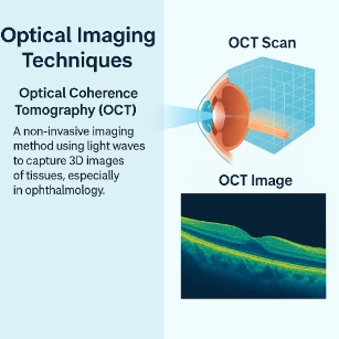
Optical coherence tomography, often shortened to OCT, is a light-based imaging method that creates cross-sectional views of biological tissue. It is especially important in eye care, where it can reveal layered structures in the retina, but the same physical ideas also support imaging in skin, blood vessels, dentistry, developmental biology, and biomedical research.
This page introduces Optical Coherence Tomography as part of the wider Bio-Optics cluster. It connects Light and Optics with biomedical imaging, tissue structure, interference, photonics, data analysis, and medical diagnostics.
The key idea is that OCT uses light echoes. A beam of low-coherence light is directed toward tissue. Some light is reflected or scattered back from different depths. By comparing this returning light with light from a reference path, the system can estimate where reflections came from and build a depth-resolved image. In this way, OCT lets light act like a gentle probe of internal microstructure.
Learning Pathway Within the Bio-Optics Cluster
This page operates as an essential cross-sectional tissue imaging module within your Bio-Optics architecture. Use the non-duplicative navigation path map below to review the entire cluster module:
Learn how fluorescent molecules, dyes, antibodies, and proteins make selected biological structures glow for imaging and analysis.
Optical Coherence Tomography
Current page. Understand how reflected light and interference create cross-sectional images of biological tissues, especially in eye and medical imaging.
See how absorption, scattering, fluorescence, spectroscopy, OCT, endoscopy, and optical sensors support diagnostic measurement.
What Optical Coherence Tomography Really Means
Optical coherence tomography is a tomographic imaging method. The word tomography means imaging by slices or sections. Instead of showing only the surface, OCT can produce a cross-sectional image that reveals structures below the visible surface of semi-transparent or weakly scattering tissue.
OCT is sometimes compared with ultrasound. Ultrasound sends sound waves into tissue and measures echoes. OCT sends light into tissue and analyses weak returning optical signals. Because light has much shorter wavelengths than sound, OCT can provide very fine structural detail, although it usually does not penetrate as deeply as ultrasound in highly scattering tissue.
This makes OCT especially useful when high-resolution imaging near the surface is needed. The eye is a major example because the transparent parts of the eye allow light to reach the retina.
Optical coherence tomography uses reflected light and interference to build cross-sectional images of tissue layers, especially in eye imaging and biomedical research.
To master the physics of optical range gating with quantitative rigor, undergraduate students must explore how the temporal coherence properties of a light source govern sub-surface axial profiling.
Michelson Interferometry and the Coherence Gate
At its operational core, an OCT system utilizes a classic Michelson interferometer illuminated by a broadband, low-coherence light source. The emission beam is split into a reference arm path and a sample arm path. When light returning from the sample tissue recombines with light from the reference mirror at the detector, the resulting interference signal modulated by a path mismatch Δz depends directly on the complex degree of temporal coherence γ(Δz).
Because the light source has a broad spectral bandwidth, the waves maintain a stable phase relationship only over an incredibly short distance. This distance defines the axial coherence length lc, which functions as an un-cut optical “coherence gate”:
Where λ0 represents the central wavelength of the source and Δλ tracks its full-width at half-maximum (FWHM) spectral bandwidth. When light backscatters from a microscopic tissue layer, a strong interference signal is generated only if the distance it traveled matches the reference arm distance within the narrow boundary of lc. This property allows OCT to separate axial depth coordinates without needing to cut or alter the specimen.
Fourier-Domain Axial Reconstruction
In modern Fourier-domain systems (including spectral-domain and swept-source configurations), the reference mirror remains completely fixed. Instead of physically moving components to track matching depths, the system records the combined interference spectrum I(ω) across different optical frequencies. According to the Wiener-Khinchin theorem, the frequency-dependent power spectrum of this combined light field forms a Fourier transform pair with its spatial autocorrelation function. The cross-interference term recorded by a spectrometer array can be expressed mathematically as:
Where S(ω) is the source spectral density, Rs(z) tracks the depth-dependent backscattering profile of the tissue, n matches the sample refractive index, and c is the speed of light in vacuum. Applying an inverse Fourier transform directly to this frequency-dependent spectrum resolves the spatial frequency modulations into a clean, real-time spatial depth profile (an A-scan).
The Basic OCT Idea: Optical Echoes
When light enters tissue, some of it travels deeper, while some is reflected or scattered backward from boundaries between structures. These weak returning signals carry information about internal layers.
However, the returning light is extremely weak and arrives from different depths. OCT solves this by using interferometry. It compares light from the tissue with light from a known reference path. Interference occurs only when the path lengths match within the coherence length of the light source. The result is depth information. By scanning across the tissue, OCT builds a two-dimensional cross-section or a three-dimensional volume.
Term
Meaning
Role in OCT
Coherence
How well light waves maintain a phase relationship
Controls how interference can occur
Low coherence
Short range over which interference remains strong
Allows depth selection
Reference arm
Known optical path with a mirror or reference reflector
Provides comparison light
Sample arm
Path where light enters tissue
Collects reflections from internal structures
Interference signal
Combined signal from reference and sample light
Reveals depth-resolved information
Main Parts of an OCT System
An OCT system combines light sources, optics, interferometry, scanning, detectors, and image processing. The details vary between instruments, but the core components are similar.
Component
Main Role
Student-Friendly Meaning
Low-coherence light source
Provides broadband or short-coherence light
Creates depth-selective interference
Beam splitter or fibre coupler
Divides light into reference and sample paths
Sends light along two routes
Reference arm
Reflects light from a known path
Provides a timing and phase comparison
Sample arm
Directs light into biological tissue
Collects echoes from tissue layers
Objective optics
Focuses light onto the tissue
Controls lateral detail and imaging area
Detector or spectrometer
Records interference signals
Turns optical information into data
Scanning system
Moves the beam across the sample
Builds cross-sections and volumes
Computer and software
Reconstructs and displays images
Transforms signals into tissue maps
A-Scans, B-Scans, and 3D OCT
OCT images are built from different kinds of scans. Understanding these scan types helps students connect the physics of light echoes with the image seen on a screen.
Scan Type
Meaning
Simple Description
A-scan
Axial depth scan
Shows reflection strength versus depth at one position
B-scan
Cross-sectional image
Combines many A-scans across a line
Volume scan
Three-dimensional dataset
Combines many B-scans across an area
En face view
Slice parallel to the tissue surface
Shows a layer viewed from above
An A-scan is like one vertical line of depth information. A B-scan is like a slice through tissue. A volume scan extends this idea into three dimensions.
Axial and Lateral Resolution Decoupling
A defining physical advantage of OCT is that its structural resolution is split into two independent directions. In standard optical microscopy, improving axial depth resolution requires opening the focus angle wider, which severely locks the sample’s depth of field. OCT solves this bottleneck through its interferometric layout:
Resolution Direction
Physical Axis
Primary Hardware Dependency
Diagnostic Impact
Axial Resolution
Depth direction (z-axis)
Light source bandwidth and coherence properties
Separates microscopic tissue boundaries and layered structural thicknesses cleanly.
Lateral Resolution
Side-by-side surface (x-y axis)
Objective focusing optics and numerical aperture (NA)
Determines the minimum width required to resolve adjacent cellular features on the surface.
Temporal Resolution
Time profile
High-speed photodiode arrays and tuning sweep rates
Minimizes motion blurring, enabling live ratiometric vascular flow scans.
Time-Domain versus Fourier-Domain Advancements
OCT systems have progressed through multiple architectural design generations to optimize speed and sensitivity:
Time-Domain OCT (TD-OCT): The earliest design generation. The reference mirror is physically translated back and forth over a mechanical tracking track to trace matching reflection distances. Because mechanical scanning is relatively slow, this configuration is highly vulnerable to patient motion blurring during standard retinal scanning.
Spectral-Domain OCT (SD-OCT): A major architectural advancement. The reference mirror is locked in a fixed position. The overlapping sample and reference beams pass through a high-rejection grating onto a stationary spectrometer camera array. By reading the spatial modulations of the spectrum, the instrument processes depth datasets instantaneously without moving parts.
Swept-Source OCT (SS-OCT): A modern, high-speed configuration. It employs a rapidly tunable narrow-band laser source that sweeps continuously across near-infrared wavelengths. A high-speed photodiode array records the resulting modulations over time, delivering deep tissue penetration with minimal light loss.
Physical Constraints: Speckle Noise and Optical Scattering boundaries
While near-infrared light paths bypass many absorption bands in blood and water, two main physical properties limit how deep an OCT scan can read:
Limitation Class
Physical Optical Cause
Practical Image Impact
Coherent Speckle
Random wave phase variations produced by backscattering across cellular networks.
Creates a grainy texture that can obscure fine, low-contrast structural features.
Multiple Scattering Distortion
Photons scatter multiple times inside dense tissues before returning to the system.
Scatters waves away from the coherence gate axis, creating a deep background noise floor.
Geometric Shadowing
Highly absorbing or dense structures (like blood vessels or melanin) block passing light.
OCT occupies a special position among imaging technologies. It offers finer structural detail than many deep-body imaging methods, but it usually has shallower penetration depth.
Method
Uses
Typical Strength
Typical Limitation
Brightfield microscopy
Thin samples, stained slides, cells
High detail in prepared samples
Usually requires thin or accessible specimens
Fluorescence imaging
Molecular labels and glowing markers
High molecular contrast
Requires labels or natural fluorescence
OCT
Cross-sectional tissue microstructure
Non-invasive layered imaging near surfaces
Limited depth in strongly scattering tissue
Ultrasound
Deeper soft-tissue imaging
Good penetration and real-time imaging
Lower resolution than OCT in many near-surface uses
MRI
Deep-body soft-tissue imaging
Excellent internal body contrast
More expensive, slower, and lower microscopic detail
CT
Bone, lung, trauma, internal structure
Strong 3D anatomical imaging
Uses ionising radiation
Ophthalmology and Beyond: Clinical and Engineering Arenas
Ophthalmology is the most prominent medical application for OCT. Because ocular structures are naturally clear and arranged in distinct layers, the instrument can easily scan through the cornea and lens to map out the microscopic tissue bands of the retina. This capability makes it indispensable for monitoring subtle structural changes over time. Beyond ophthalmology, OCT principles are widely used across multiple biomedical fields:
Dermatology Surface Tracking
Maps out near-surface skin layers to help researchers observe wound-healing dynamics and measure epidermal thickness variations non-invasively.
Intravascular Plaque Assessment
Miniature fiber-optic probes are built into clinical catheters to perform internal cardiovascular scans, mapping out arterial wall microstructures and lipid plaque boundaries.
Dental Micro-Crack Diagnostics
Scans dental enamel to detect early subsurface cracks and monitor mineral decay layers before changes are visible on the surface.
Tissue Engineering Monitoring
Scans engineered cellular scaffolds over time, providing researchers with non-destructive, layered growth data without ruining the sample.
OCT Imaging Workflow
A typical OCT imaging process follows a clear workflow from optical scanning to interpretation.
Step
What Happens
Why It Matters
Prepare the subject or sample
Position the eye, tissue, or specimen
Reduces motion and improves focus
Send light into the sample
Low-coherence light enters the tissue
Creates depth-sensitive optical echoes
Collect returning light
Backscattered or reflected light returns to the system
Carries information about internal layers
Compare with reference light
Interference reveals depth information
Converts optical path differences into signals
Scan across the tissue
Many A-scans are collected
Builds cross-sectional or volumetric data
Reconstruct image
Software processes signals into images
Creates B-scans, layer maps, or volumes
Interpret carefully
Images are assessed with context and expertise
Avoids overreading artefacts or noise
Modern workflows convert raw interferometric signals directly into digitized pixel arrays. This digitization enables automated tracking software to run edge-detection routines that quickly calculate tissue layer thicknesses, seamlessly connecting advanced optics hardware with the processing pipelines of Data Science and Analytics.
Quick Check: Optical Coherence Tomography
Quick Check: OCT Basics
Q1. What does OCT use to create cross-sectional tissue images?
OCT combines low-coherence broadband light sources with a reference interferometer path to turn weak backscattered light echoes into depth-resolved cross-sectional images.
Q2. Why is OCT often described as an optical analogue to ultrasound?
Both modalities track returning reflection signals from internal structural boundaries. Ultrasound measures acoustic sound wave reflections, whereas OCT records optical light wave reflections.
Q3. What is the distinction between an A-scan and a B-scan?
An A-scan is a single one-dimensional depth scan at a specific point on the tissue. A B-scan combines a series of adjacent A-scans across a line to form a two-dimensional cross-sectional slice.
Q4. Why is OCT uniquely suited for retinal diagnostics?
Ocular tissues are naturally transparent, allowing light to reach the back of the eye easily. This clear optical access lets OCT map out distinct retinal layers without needing to cut tissue.
Numerical Practice: Interferometry Calculations
Numerical Problems and Solutions
1. An OCT system uses an infrared light source centered at a wavelength of 850 nm. Calculate the energy of a single excitation photon.
Apply Planck’s equation:
$$E = \frac{hc}{\lambda}$$
Convert the wavelength to base meters ($850\text{ nm} = 850 \times 10^{-9}\text{ m}$):
Answer: The energy of the photon is approximately 2.34 × 10⁻¹⁹ Joules.
2. A Fourier-domain B-scan line is composed of 600 individual A-scans. If the spectrometer camera registers an acquisition speed of 20 μs per individual depth scan, calculate the total line scan time.
Multiply the individual scan time by the total number of scans in the line:
Answer: Generating the complete B-scan slice takes exactly 0.012 s (or 12 ms).
3. An initialized scan axis registers an effective pixel size step of 5 μm along the depth direction. An cross-sectional retinal layer boundary spans exactly 24 pixels. Estimate the thickness of the layer.
Multiply the pixel span count by the calibrated axial step factor:
Answer: The structural layer thickness is exactly 120 μm.
4. A volumetric 3D diagnostic dataset contains exactly 300 adjacent B-scan cross-sections. If each discrete slice line is compiled using 500 individual A-scans, determine the total number of depth profiles in the volume.
Multiply the number of slices by the number of scans per slice:
Answer: The 3D volume scan contains exactly 150,000 A-scans.
5. A light signal drops from an initial count of 10,000 down to 2500 after passing through a highly scattering skin layer. Calculate the remaining intensity fraction.
Divide the exiting intensity signal count by the initial input level:
Answer: A fraction of 0.25 (or 25%) of the original light signal remains unscattered.
6. An optical scanner sweeps a 6 mm horizontal path line across a specimen using 1200 individual A-scan steps. Determine the lateral spacing between adjacent points.
Divide the total scan line length by the number of step coordinates:
Optical coherence tomography stands as a major triumph in modern bio-optics, showing how low-coherence light interference can map out hidden tissue layers non-invasively. By tracking weak backscattered light echoes and comparing them with a known reference path, the instrument bypasses classical depth bottlenecks. This capability allows it to deliver micrometer-scale axial scans without needing to physically slice the sample. While physical boundaries like coherent speckle noise and limited penetration depths in dense tissues require careful calibration, its decoupling of axial and lateral resolution makes OCT an essential tool for tracking live structures across ophthalmology, cardiology, and biological discovery.
Reflection Question
If OCT can turn weak reflections from tissue into a layered image, what does this teach us about the hidden information carried by light?