
Robotics and quantum computing converge at the frontier of computational complexity. Modern autonomous machines rely on classical von Neumann processors for sensor perception, real-time feedback control, and low-level actuation. However, many high-level planning and decision-making problems in robotics become computationally intractable as system dimensionality, operational horizons, or fleet sizes scale.
The computational bottleneck is not in executing motor commands or high-frequency sensor updates—those demand deterministic, sub-millisecond physical response times that classical embedded microcontrollers execute efficiently. Instead, computational explosions emerge in non-convex, NP-hard reasoning domains, including high-dimensional motion planning, multi-robot swarm task allocation, combinatorial route scheduling, and factor-graph optimization.
As robotic environments expand, the underlying configuration and state spaces grow exponentially. Quantum information science explores whether physical quantum phenomena—specifically superposition, quantum entanglement, and constructive wave interference—can explore these massive solution landscapes more effectively than classical heuristic search.
If practical quantum advantage materializes, it will integrate into robotics by assisting high-performance computing centers in resolving large-scale combinatorial scheduling, fleet logistics, and global trajectory synthesis, while leaving real-time physical joint actuation to classical embedded hardware.
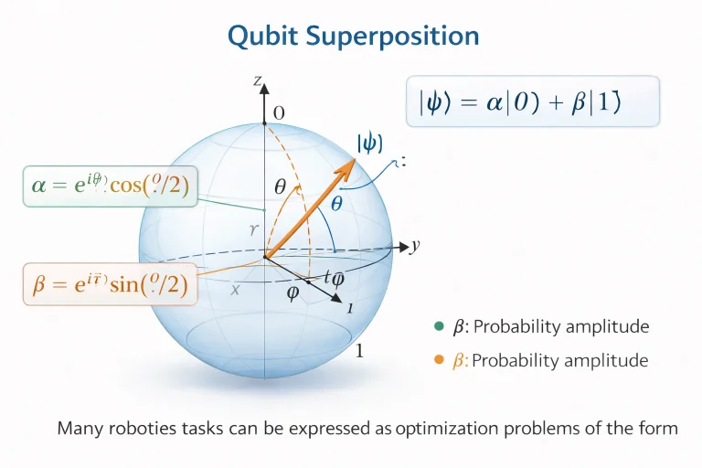
This geometric model illustrates a single quantum bit (qubit) state vector on the unit Bloch sphere. Unlike a classical binary digit constrained to discrete states 0 or 1, a qubit exists as a continuous superposition across complex probability amplitudes \(\alpha\) and \(\beta\). Unitary quantum gate operations rotate this state vector continuously across the sphere's surface, manipulating relative phases to achieve constructive interference before state measurement collapses the qubit into a classical binary value.
Interactive Quick Review: Quantum Advantage & Superposition
Test your understanding of high-level quantum optimization versus low-level real-time control before exploring qubit mechanics:
1. Why is quantum computing envisioned for high-level planning rather than direct low-level motor control?
Answer: Low-level motor control loops require deterministic sub-millisecond execution that classical microcontrollers handle efficiently. Quantum processors excel at exploring exponential combinatorial search spaces (such as multi-robot scheduling or global path planning) where classical algorithms suffer from computational runtime explosions.
2. What quantum phenomenon allows a qubit to represent multiple states simultaneously prior to measurement?
Answer: Quantum superposition, which allows a qubit state \(|\psi\rangle = \alpha |0\rangle + \beta |1\rangle\) to exist as a linear combination of basis vectors in a complex Hilbert space until physical measurement collapses it into a definite classical state.
Glossary of Key Terminology
Essential mathematical, physical, and algorithmic concepts defining quantum computing, state spaces, and quantum-assisted robotics:
Quantum Bits and the Bloch Sphere Representation
A classical computational bit holds a deterministic binary state \(b \in \{0, 1\}\). A quantum bit (qubit) is a two-level quantum mechanical system represented mathematically as a normalized unit vector in a two-dimensional complex Hilbert space \(\mathcal{H}_2 \cong \mathbb{C}^2\):
$$|\psi\rangle = \alpha |0\rangle + \beta |1\rangle = \begin{bmatrix} \alpha \\ \beta \end{bmatrix}$$where \(\alpha, \beta \in \mathbb{C}\) denote complex probability amplitudes satisfying the normalization condition derived from the Born rule:
$$\langle \psi | \psi \rangle = |\alpha|^2 + |\beta|^2 = 1$$Upon physical measurement in the computational \(Z\)-basis, the superposition collapses into a definite classical state with probabilities:
$$P(0) = |\alpha|^2, \quad P(1) = |\beta|^2$$Geometrically, neglecting an unobservable global phase factor \(e^{i\delta}\), any pure single-qubit state can be parameterized on the unit Bloch sphere using polar angle \(\theta \in [0, \pi]\) and azimuthal phase angle \(\phi \in [0, 2\pi)\):
$$|\psi\rangle = \cos\left(\frac{\theta}{2}\right) |0\rangle + e^{i\phi} \sin\left(\frac{\theta}{2}\right) |1\rangle$$The vector \(\vec{r} = [\sin\theta \cos\phi, \sin\theta \sin\phi, \cos\theta]^T\) identifies a point on the surface of the sphere, illustrating how single-qubit quantum gates correspond to geometric rotations \(\mathbf{R}_{\hat{n}}(\theta) \in SO(3)\).
Multi-Qubit Systems and Exponential State Space Scaling
When multiple qubits interact, their joint state space is formed via the tensor product of individual Hilbert spaces. For a composite register of \(n\) qubits, the state space expands into a \(2^n\)-dimensional complex vector space \(\mathcal{H}^{\otimes n}\):
$$|\Psi\rangle = \sum_{x \in \{0, 1\}^n} c_x |x\rangle = c_{0\dots00}|0\dots00\rangle + c_{0\dots01}|0\dots01\rangle + \dots + c_{1\dots11}|1\dots11\rangle$$where \(\sum_{x} |c_x|^2 = 1\). While a classical register of \(n\) bits stores exactly one of \(2^n\) configurations at any instant, an \(n\)-qubit quantum register stores a superposition encompassing all \(2^n\) configurations simultaneously across \(2^n\) complex amplitudes.
This exponential scaling (\(\dim(\mathcal{H}) = 2^n\)) allows quantum processors to represent massive combinatorial spaces with compact hardware registers. For example, a 60-qubit register represents \(2^{60} \approx 1.15 \times 10^{18}\) simultaneous basis configurations—a search space that exceeds the memory capacity of classical supercomputers.
Quantum Approximate Optimization (QAOA) for Combinatorial Logistics
Many multi-robot fleet planning tasks reduce to Quadratic Unconstrained Binary Optimization (QUBO) problems or Ising spin-glass models:
$$\min_{\mathbf{x} \in \{0, 1\}^n} \mathbf{x}^T \mathbf{Q} \mathbf{x} + \mathbf{c}^T \mathbf{x}$$These formulations model problems such as warehouse robot package dispatching, multi-agent collision-free routing, and battery charging schedules.
The Quantum Approximate Optimization Algorithm (QAOA) solves these combinatorial problems using shallow variational circuits. The classical objective function is mapped into a diagonal cost Hamiltonian \(\hat{H}_C\) by mapping binary variables \(x_i \in \{0, 1\}\) to Pauli spin operators \(\hat{Z}_i \in \{+1, -1\}\):
$$x_i \to \frac{\mathbf{I} - \hat{Z}_i}{2}$$A QAOA circuit applies \(p\) alternating layers of cost and mixing Hamiltonians onto an initial uniform superposition state \(|+\rangle^{\otimes n}\):
$$|\boldsymbol{\gamma}, \boldsymbol{\beta}\rangle = \prod_{k=1}^{p} \left( e^{-i \beta_k \hat{H}_M} e^{-i \gamma_k \hat{H}_C} \right) |+\rangle^{\otimes n}$$where:
- \(\hat{H}_C\): Problem cost Hamiltonian encoding the robot optimization objective.
- \(\hat{H}_M = \sum_{j=1}^{n} \hat{X}_j\): Transverse-field mixing Hamiltonian driving transitions across basis states.
- \(\boldsymbol{\gamma}, \boldsymbol{\beta} \in \mathbb{R}^p\): Variational rotation parameters tuned iteratively by a classical optimizer (e.g., COBYLA, Adam) to minimize the expectation value: $$\min_{\boldsymbol{\gamma}, \boldsymbol{\beta}} \langle \boldsymbol{\gamma}, \boldsymbol{\beta} | \hat{H}_C | \boldsymbol{\gamma}, \boldsymbol{\beta} \rangle$$
Quantum Search & Motion Planning Graph Complexity
In robot motion planning, finding collision-free paths through high-dimensional configuration spaces (\(C\)-space) often requires searching massive discrete roadmaps or spatial grid graphs, as discussed in Path Planning Algorithms for Robots.
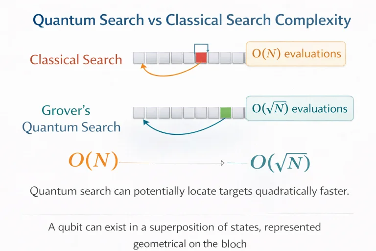
For an unsorted discrete search space containing \(N\) candidate state configurations, classical search requires \(\mathcal{O}(N)\) evaluations in the worst case and \(N/2\) on average. Grover’s algorithm constructs a quantum oracle \(\mathbf{U}_\omega\) that inverts the phase of valid solution states (\(|\omega\rangle \to -|\omega\rangle\)), followed by the Grover diffusion operator \(\mathbf{U}_s = 2|s\rangle\langle s| - \mathbf{I}\) that reflects amplitudes about their mean.
By repeatedly applying the Grover iteration operator \(\mathbf{G} = \mathbf{U}_s \mathbf{U}_\omega\), the target state probability amplitude grows constructively. The optimal number of iterations scales as:
$$R \approx \left\lfloor \frac{\pi}{4} \sqrt{\frac{N}{M}} \right\rfloor$$where \(M\) is the number of marked valid solutions. For \(M = 1\), this yields a quadratic speedup of \(\mathcal{O}(\sqrt{N})\), reducing a search over \(16,000,000\) states from sixteen million classical queries to approximately \(3,142\) quantum iterations.
Engineering Challenges & Technical Solutions
Bridging quantum information processing and physical robotics requires resolving several fundamental electromechanical, physical, and systems challenges:
The Challenge: Leading quantum computing platforms (superconducting transmon qubits and semiconductor spin qubits) require dilution refrigerators operating near absolute zero (\(15\text{ millikelvin}\)). This equipment is bulky, heavy, and power-intensive, making onboard mounting on mobile robots impossible in the near term.
- Hybrid Classical-Quantum Cloud Architectures: Mobile robots run real-time control locally while offloading large optimization problems to remote quantum datacenters via 5G or Wi-Fi links.
- Room-Temperature Trapped-Ion & Photonic Processors: Research into room-temperature photonic circuits and neutral-atom processors may eventually enable compact, field-deployable quantum co-processors.
The Challenge: Current Noisy Intermediate-Scale Quantum (NISQ) processors experience gate errors and decoherence within microseconds (\(T_1, T_2 < 200\ \mu\text{s}\)). Thermal vibrations and electromagnetic noise destroy superposition states before deep optimization circuits can finish executing.
- Zero-Noise Extrapolation (ZNE): Artificially scaling hardware noise over multiple runs and extrapolating results back to the zero-noise limit mathematically to recover optimization signals.
- Shallow-Depth Variational Algorithms: Designing low-depth QAOA and VQE circuits parameterized to complete execution well within the physical \(T_1\) relaxation window.
The Challenge: Measuring a multi-qubit register collapses continuous probability amplitudes into a single binary string. Reconstructing continuous joint trajectory distributions requires thousands of repeated quantum circuit executions (shots), introducing readout latencies that exceed real-time control loop deadlines.
- Shadow Tomography & Classical Shadows: Efficiently capturing randomized Pauli measurements to estimate multiple trajectory observables using logarithmic quantum shot budgets.
- Asynchronous Decoupled Execution: Allowing the classical robot controller to interpolate intermediate trajectories while the quantum co-processor evaluates long-horizon path updates in the background.
The Challenge: Physical robotic joints operate on continuous spatial manifolds (\(\mathbb{R}^n\) and \(SE(3)\)). Mapping continuous non-linear kinematics into discrete two-level qubit registers requires fine discretization that quickly exhausts available physical qubits.
- Continuous-Variable (CV) Quantum Computing: Using photonic qumodes and continuous quantum states (position and momentum quadratures) to match continuous robotic state spaces directly.
- Quantum-Inspired Tensor Networks: Running classical tensor network algorithms (such as Matrix Product States) on classical GPUs to simulate high-dimensional parameter spaces without requiring physical quantum hardware.
Hybrid Classical–Quantum Robotics Architectures
Practical near-term deployments will rely on hybrid classical–quantum architectures that divide computational responsibilities based on hardware strengths:
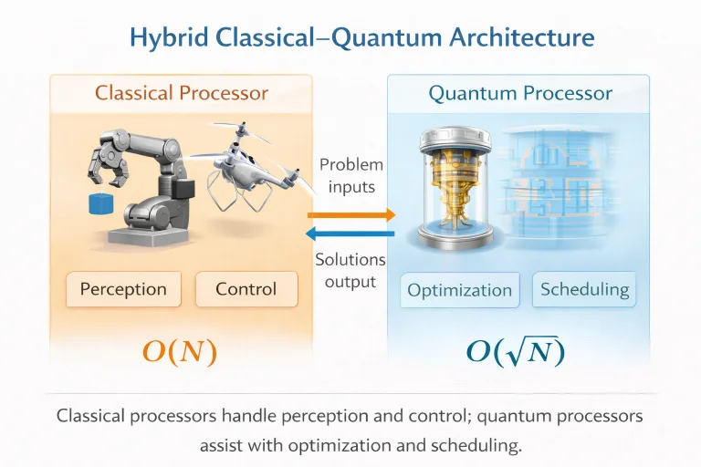
The system allocates tasks across distinct computing tiers:
- Classical Onboard Edge Layer: High-bandwidth sensor acquisition (cameras, LiDAR, IMU), SLAM state estimation, and 1 kHz deterministic motor PID/computed torque control loops running on embedded processors, as covered in Real-Time Embedded Systems in Robotics.
- Classical Edge Server Layer: Intermediate coordinate transformation caching (TF2), local trajectory obstacle checking, and mapping continuous states to binary optimization matrices.
- Quantum Cloud Co-Processor (QPU): Receiving mapped Hamiltonians, executing variational quantum optimization circuits (QAOA, Quantum Annealing), and returning low-cost discrete assignments (such as optimal multi-agent routing graphs) back to the classical planners.
Interactive Quick Review: Grover, QAOA & Hybrid Systems
Reinforce key concepts regarding quadratic search speedups, hybrid architectures, and quantum decoherence limits before reviewing the FAQ:
1. How does Grover’s quantum search algorithm achieve a quadratic speedup over classical unsorted search?
Answer: By manipulating quantum superposition and constructive amplitude amplification, Grover's algorithm locates a target configuration in \(\mathcal{O}(\sqrt{N})\) iterations compared to the classical worst-case \(\mathcal{O}(N)\) linear search.
2. What is the role of the cost Hamiltonian \(\hat{H}_C\) in the Quantum Approximate Optimization Algorithm (QAOA)?
Answer: The cost Hamiltonian \(\hat{H}_C\) encodes the mathematical objective function (such as energy consumption or trajectory travel time) into quantum energy levels, allowing phase rotation operations to penalize high-cost states.
External References and Further Reading
To explore quantum algorithms, quantum information processing, and frontier quantum optimization research, consult the following authoritative sources:
- IBM Quantum & Qiskit SDK – Open-source quantum computing framework providing tools to build, simulate, and execute QAOA and Grover search algorithms on real hardware.
- Google Quantum AI Research – Research platform publishing advances in NISQ hardware, fault-tolerant quantum error correction, and quantum optimization benchmarks.
- Quantum Computation and Quantum Information (Nielsen & Chuang) – The standard academic textbook detailing linear algebra foundations, quantum circuits, and algorithmic complexity limits.
Frequently Asked Questions about Robotics and Quantum Computing
Will quantum processors ever be mounted directly onto mobile robots?
In the near term, direct onboard mounting is physically unfeasible because superconducting quantum processors require bulky cryogenic dilution refrigerators operating near absolute zero (\(15\text{ millikelvin}\)). Quantum robotics utilizes offboard cloud connections, offloading heavy optimization tasks to quantum datacenters while classical embedded processors execute local real-time motor control.
What is the difference between a NISQ processor and a fault-tolerant quantum computer?
Noisy Intermediate-Scale Quantum (NISQ) devices contain tens to hundreds of physical qubits without active error correction, limiting circuit depth due to noise. Fault-tolerant quantum computers use thousands of physical qubits to form a single error-corrected "logical qubit," allowing execution of arbitrarily long algorithms without decoherence.
How does a quantum computer represent \(2^n\) state configurations using only n qubits?
Through quantum superposition and tensor product state spaces. An \(n\)-qubit quantum register state \(|\psi\rangle = \sum c_i |i\rangle\) is a complex linear combination of \(2^n\) orthogonal basis states, allowing a single quantum state vector to hold \(2^n\) probability amplitudes simultaneously.
Can quantum algorithms solve NP-hard robotics problems in polynomial time?
Quantum computers are not believed to solve NP-hard problems (like the Travelling Salesperson Problem) in polynomial time. However, algorithms like QAOA and Quantum Annealing offer polynomial or quadratic heuristics that may find higher-quality approximate solutions much faster than classical heuristics for massive fleet sizes.
What is quantum decoherence, and why is it a bottleneck for robotics applications?
Quantum decoherence occurs when environmental thermal vibrations or electromagnetic interference interact with qubits, causing superpositions to collapse prematurely into classical noise. Because robotic optimization routines require deep quantum circuits, decoherence destroys computation before optimal trajectory solutions can be extracted.
What are "quantum-inspired" classical algorithms?
Quantum-inspired algorithms are classical algorithms running on standard GPUs or TPUs that borrow mathematical principles developed for quantum mechanics (such as tensor network contractions or simulated annealing with quantum fluctuations), delivering significant speedups without requiring physical quantum hardware.
How could quantum computing improve Simultaneous Localization and Mapping (SLAM)?
Large-scale SLAM builds massive non-linear pose graphs with thousands of historical robot poses and landmark constraints. Quantum matrix inversion algorithms (such as HHL) and quantum graph optimization could theoretically accelerate solving large sparse linear systems underlying factor-graph SLAM optimizations.
What career paths prepare students for research at the intersection of robotics and quantum AI?
Students should pursue dual specialties in quantum information science, theoretical computer science, operations research, and autonomous systems control, building expertise in linear algebra, C++, Python, and quantum SDKs (Qiskit, Cirq, PennyLane).
End-of-Page Exercises: Review, Thought-Provoking & Engineering Problems
Section 1: Foundational Review Questions & Answers
1. What equation describes the normalized quantum state \(|\psi\rangle\) of a single qubit in superposition?
Answer: \(|\psi\rangle = \alpha |0\rangle + \beta |1\rangle\), subject to normalization constraint \(|\alpha|^2 + |\beta|^2 = 1\).
2. How many simultaneous basis states exist in the Hilbert space of an n-qubit register?
Answer: \(2^n\) basis states, expanding exponentially with the number of qubits.
3. What algorithmic time complexity is achieved by Grover’s search algorithm compared to classical unsorted search \(\mathcal{O}(N)\)?
Answer: \(\mathcal{O}(\sqrt{N})\), delivering a quadratic reduction in oracle query complexity.
4. What does QAOA stand for, and what class of robotics problems does it address?
Answer: Quantum Approximate Optimization Algorithm; it addresses combinatorial optimization problems such as multi-robot task allocation, route scheduling, and graph partitioning.
5. In QAOA parameter optimization, what roles are played by \(\hat{H}_C\) and \(\hat{H}_M\)?
Answer: \(\hat{H}_C\) is the cost Hamiltonian that encodes the objective function, and \(\hat{H}_M\) is the mixing Hamiltonian that enables state space exploration through quantum transitions.
6. What division of labor characterizes a hybrid classical–quantum robotics architecture?
Answer: Classical processors execute high-speed perception, sensing, and real-time motor control loops, while quantum co-processors execute large-scale, offloaded combinatorial optimization routines.
7. What geometric sphere represents single-qubit pure state superpositions?
Answer: The Bloch sphere.
8. Name four specific robotics domains that exhibit combinatorial optimization structures suitable for quantum exploration.
Answer: Multi-robot task allocation, global trajectory optimization, swarm fleet coordination, and factor-graph SLAM optimization.
9. What environmental physical factors cause quantum decoherence in quantum hardware?
Answer: Thermal fluctuations, stray electromagnetic radiation, magnetic fields, and atomic material defects.
10. Name five university mathematics and physics topics foundational to quantum robotics study.
Answer: Linear algebra (complex vector spaces), probability amplitude theory, eigenvalues/operators, optimization theory, and basic quantum mechanics.
Section 2: Analytical & Thought-Provoking Questions
1. Why is the No-Cloning Theorem in quantum mechanics a major challenge when attempting to save intermediate states during quantum path planning?
Answer: The No-Cloning Theorem proves mathematically that an arbitrary unknown quantum state cannot be duplicated exactly. In classical path planning (like A* or RRT), planners freely duplicate search nodes to construct branching trees. Quantum planners cannot duplicate an active superposition state, requiring unitary reversible transformations and specialized quantum memory registers (QRAM) to track search histories.
2. How does phase kickback enable Grover’s algorithm to amplify the probability amplitude of a valid collision-free trajectory configuration?
Answer: A quantum oracle flips the phase sign of the target state (\(|x\rangle \to -|x\rangle\)). The Grover diffusion operator then reflects all state amplitudes about their mean. Because the target state phase is inverted, reflecting about the mean increases its probability amplitude while decreasing non-target amplitudes, making measurement of the optimal path highly probable after \(\mathcal{O}(\sqrt{N})\) steps.
3. Why do wireless network latencies in cloud-quantum architectures restrict quantum speedups to static global planning rather than dynamic obstacle avoidance?
Answer: Cloud telemetry round-trips introduce 20–100 ms latencies. Dynamic collision avoidance requires sub-5 ms local control loops. Thus, cloud quantum processing is restricted to computing high-level global warehouse fleet schedules or pre-mission multi-agent assignments where execution delays do not trigger immediate physical collisions.
4. How can Quantum Annealing solve Quadratic Unconstrained Binary Optimization (QUBO) problems in fleet logistics?
Answer: QUBO maps binary decisions (e.g., Robot \(i\) assigned to Job \(j\)) to spin states on a physical quantum processor grid. The annealer initializes qubits in a ground state and slowly decreases transverse magnetic fields, allowing quantum tunneling to bypass high energy cost barriers and settle into global energy minima representing optimal fleet schedules.
5. What causes the measurement collapse bottleneck when reading out multi-qubit trajectory optimization results?
Answer: Measuring an \(n\)-qubit register collapses a rich \(2^n\)-dimensional superposition into a single classical binary string. Extracting optimal continuous joint trajectory profiles requires repeating the quantum circuit execution and measurement thousands of times ("shots") to reconstruct the probability distribution, introducing significant measurement readout overhead.
6. How does domain mapping convert a non-linear continuous robot manipulator configuration into a discrete quantum Hamiltonian?
Answer: Continuous joint angle spaces are discretized into \(2^k\) binary angle steps encoded across \(k\) qubits per joint. Objective cost functions (tracking error and motor energy penalty \(\|\mathbf{q} - \mathbf{q}_d\|^2 + \lambda \|\boldsymbol{\tau}\|^2\)) are converted into Pauli matrix spin operators (\(\hat{Z}_i, \hat{X}_i\)), forming a cost Hamiltonian \(\hat{H}_C\) whose lowest energy eigenvalue corresponds to the optimal trajectory.
7. Why is Parameterized Quantum Circuit (PQC) optimization vulnerable to the "barren plateau" phenomenon in deep variational algorithms?
Answer: Barren plateaus occur when partial gradients of the cost function with respect to variational parameters (\(\nabla_{\boldsymbol{\gamma}, \boldsymbol{\beta}} J\)) decay exponentially toward zero as qubit count increases. This flattens the optimization landscape, preventing classical optimizers (like gradient descent) from finding effective search directions in deep QAOA circuits.
8. How could Quantum Random Number Generators (QRNGs) improve stochastic sampling in high-dimensional RRT path planning?
Answer: Classical pseudo-random number generators (PRNGs) rely on deterministic algorithms that exhibit subtle periodicity and correlation biases, leading to non-uniform sampling coverage in complex C-spaces. QRNGs exploit fundamental quantum measurement randomness, generating truly uncorrelated uniform random points \(\mathbf{q}_{\text{rand}}\) that improve RRT space-filling efficiency.
9. In what way does Quantum Machine Learning (QML) alter the training dynamics of neural network policies in reinforcement learning?
Answer: QML replaces classical neural network layers with Quantum Neural Networks (QNNs) built from parameterized rotation gates. Quantum entanglement allows QNNs to represent non-linear state-action feature correlations using exponentially fewer parameters than classical deep networks, theoretically lowering training sample complexity for complex locomotion tasks.
10. Why do error mitigation techniques (like zero-noise extrapolation) play a vital role in current NISQ-era robotics benchmarks?
Answer: Uncorrected NISQ hardware introduces gate errors that corrupt calculated trajectory costs. Zero-noise extrapolation intentionally scales hardware noise upward across multiple experimental runs and extrapolates measured expectation values back to the zero-noise limit mathematically, recovering accurate optimization signals without full hardware error correction.
11. How can quantum walk algorithms accelerate graph exploration in unstructured multi-agent maze environments compared to classical random walks?
Answer: Classical random walks propagate diffusively through a graph with spatial spread proportional to time (\(\sqrt{t}\)). Quantum walks utilize quantum wave interference across graph edges, propagating quadratically faster with linear spatial spread proportional to \(t\), enabling mobile robot swarms to discover network exit routes faster.
12. What economic factors dictate whether industrial robot fleet operators will adopt quantum cloud optimization services?
Answer: Industrial adoption hinges on total cost of ownership versus efficiency gains. Operators will adopt quantum cloud scheduling only if the percentage reduction in fleet energy consumption, travel distance, or task completion time generates financial savings that outweigh cloud quantum compute subscription costs relative to high-performance classical solvers.
Section 3: Numerical Engineering Problems & Solutions
A quantum bit in an optimization circuit is prepared in the normalized pure state \(|\psi\rangle = \frac{\sqrt{5}}{3}|0\rangle + \beta |1\rangle\). Calculate the exact value of probability amplitude \(\beta\) (assuming \(\beta\) is a positive real number), and determine the physical measurement probabilities \(P(0)\) and \(P(1)\) expressed as exact fractions and percentages.
1. Apply the Born rule normalization condition: $$|\alpha|^2 + |\beta|^2 = 1$$ 2. Evaluate \(|\alpha|^2\): $$|\alpha|^2 = \left(\frac{\sqrt{5}}{3}\right)^2 = \frac{5}{9}$$ 3. Solve for \(|\beta|^2\) and \(\beta\): $$|\beta|^2 = 1 - \frac{5}{9} = \frac{4}{9} \Rightarrow \beta = \sqrt{\frac{4}{9}} = \frac{2}{3}$$ 4. Compute physical measurement probabilities: $$P(0) = |\alpha|^2 = \frac{5}{9} \approx 55.56\%$$ $$P(1) = |\beta|^2 = \frac{4}{9} \approx 44.44\%$$ Final Answer: Probability amplitude is \(\beta = \frac{2}{3}\); measurement probabilities are \(P(0) = \frac{5}{9}\ (55.56\%)\) and \(P(1) = \frac{4}{9}\ (44.44\%)\).
A multi-robot fleet allocation algorithm assigns 12 autonomous mobile robots across 12 delivery tasks using a quantum state encoding where each task-robot decision corresponds to a physical qubit register. Calculate the total number of physical qubits \(n\) required, compute the exact dimension \(2^n\) of the resulting Hilbert state space, and convert the state count into standard scientific notation.
1. Determine qubit register count: $$n = 12\text{ qubits}$$ 2. Compute Hilbert space dimensionality: $$\dim(\mathcal{H}) = 2^{12} = 4096\text{ basis states}$$ 3. Express in scientific notation: $$\dim(\mathcal{H}) = 4.096 \times 10^3$$ Final Answer: The register requires \(12\text{ qubits}\), representing a Hilbert state space dimension of \(4096\text{ basis states}\) (\(4.096 \times 10^3\)).
A high-dimensional robot motion planner must search through an unsorted discrete configuration space containing \(N = 16,000,000\) candidate states. Calculate the worst-case evaluations required by a classical search algorithm (\(N\)), calculate the approximate iterations required by Grover’s quantum search (\(\lfloor \frac{\pi}{4} \sqrt{N} \rfloor\)), and determine the exact algorithmic speedup factor (\(N / N_{\text{grover}}\)).
1. Classical worst-case query complexity: $$N_{\text{classical}} = 16,000,000\text{ operations}$$ 2. Evaluate square root of search space: $$\sqrt{N} = \sqrt{16,000,000} = 4000$$ 3. Compute Grover iteration count: $$N_{\text{grover}} \approx \left\lfloor \frac{\pi}{4} \times 4000 \right\rfloor = \lfloor 3141.59 \rfloor = 3141\text{ iterations}$$ 4. Determine algorithmic speedup factor: $$\text{Speedup} = \frac{N_{\text{classical}}}{N_{\text{grover}}} = \frac{16,000,000}{3141} \approx 5093.92$$ Final Answer: Grover search reduces queries from 16,000,000 down to \(3141\text{ iterations}\), delivering a \(\approx 5094\text{-fold}\) computational speedup.
A QAOA trajectory optimization circuit rotates qubit states using cost parameter \(\gamma = 0.35\pi\text{ radians}\) and mixing parameter \(\beta = 0.15\pi\text{ radians}\). Convert both parameter angles from radians to degrees, and calculate the ratio \(\gamma / \beta\).
1. Convert \(\gamma\) to degrees: $$\gamma_{\text{deg}} = 0.35 \times 180^\circ = 63.0^\circ$$ 2. Convert \(\beta\) to degrees: $$\beta_{\text{deg}} = 0.15 \times 180^\circ = 27.0^\circ$$ 3. Compute parameter ratio: $$\text{Ratio} = \frac{\gamma}{\beta} = \frac{0.35\pi}{0.15\pi} = \frac{63.0^\circ}{27.0^\circ} = \frac{7}{3} \approx 2.3333$$ Final Answer: Variational parameter angles are \(\gamma = 63.0^\circ\) and \(\beta = 27.0^\circ\), with a ratio of \(2.333\).
A quantum multi-robot coordination system prepares an entangled Bell state \(|\Phi^+\rangle = \frac{1}{\sqrt{2}}|00\rangle + \frac{1}{\sqrt{2}}|11\rangle\). Calculate the physical measurement probability of observing state \(|00\rangle\), state \(|11\rangle\), and state \(|01\rangle\).
1. Compute measurement probability for \(|00\rangle\): $$P(00) = \left|\frac{1}{\sqrt{2}}\right|^2 = \frac{1}{2} = 0.50 \quad (50.0\%)$$ 2. Compute measurement probability for \(|11\rangle\): $$P(11) = \left|\frac{1}{\sqrt{2}}\right|^2 = \frac{1}{2} = 0.50 \quad (50.0\%)$$ 3. Compute measurement probability for \(|01\rangle\): $$P(01) = |0|^2 = 0.00 \quad (0.0\%)$$ Final Answer: Measurement probabilities are \(P(00) = 50.0\%\), \(P(11) = 50.0\%\), and \(P(01) = 0.0\%\) (demonstrating maximal quantum correlation).
To manage a swarm of \(N_{\text{swarm}} = 20\text{ autonomous drones}\), a quantum coordinator allocates \(k = 3\text{ qubits}\) per drone to represent 8 discrete spatial altitude corridors (\(2^3 = 8\)). Calculate the total required system qubits \(N_{\text{qubits}}\), and compute the dimensionality of the swarm configuration Hilbert space \(2^{N_{\text{qubits}}}\).
1. Calculate total qubit register requirement: $$N_{\text{qubits}} = N_{\text{swarm}} \times k = 20 \times 3 = 60\text{ qubits}$$ 2. Calculate state space dimensionality: $$\dim(\mathcal{H}) = 2^{60} \approx 1.1529 \times 10^{18}\text{ basis configurations}$$ Final Answer: The swarm allocator requires \(60\text{ qubits}\), representing a Hilbert state space dimension of \(\approx 1.15 \times 10^{18}\text{ simultaneous configurations}\).
A superconducting quantum processor executing a robotic trajectory optimization circuit has a characteristic coherence relaxation time \(T_1 = 120\ \mu\text{s}\). The executed QAOA circuit consists of 40 sequential two-qubit gate layers, where each gate layer execution takes \(t_{\text{gate}} = 2.5\ \mu\text{s}\). Calculate total circuit execution time \(T_{\text{circuit}}\) and determine the remaining coherence execution margin \(T_1 - T_{\text{circuit}}\).
1. Compute total circuit execution duration: $$T_{\text{circuit}} = 40\text{ layers} \times 2.5\ \mu\text{s/layer} = 100.0\ \mu\text{s}$$ 2. Verify against coherence threshold: $$100.0\ \mu\text{s} \le 120.0\ \mu\text{s} \quad (\text{Execution Feasible})$$ 3. Compute remaining safety headroom: $$\text{Margin} = T_1 - T_{\text{circuit}} = 120.0\ \mu\text{s} - 100.0\ \mu\text{s} = 20.0\ \mu\text{s}$$ Final Answer: Total circuit runtime is \(100.0\ \mu\text{s}\), leaving a \(20.0\ \mu\text{s}\) coherence safety margin.
A cloud-connected mobile robot dispatches a 50-variable task allocation matrix to a remote quantum datacenter over 5G. Upstream transmission takes \(t_{\text{net}} = 18\text{ ms}\), quantum circuit compilation takes \(t_{\text{compile}} = 12\text{ ms}\), QPU execution (1,000 measurement shots) takes \(t_{\text{qpu}} = 15\text{ ms}\), and downstream result transmission takes \(t_{\text{return}} = 18\text{ ms}\). Calculate the total round-trip optimization latency \(T_{\text{latency}}\) in milliseconds.
1. Sum all sequential pipeline latency components: $$T_{\text{latency}} = t_{\text{net}} + t_{\text{compile}} + t_{\text{qpu}} + t_{\text{return}}$$ $$T_{\text{latency}} = 18\text{ ms} + 12\text{ ms} + 15\text{ ms} + 18\text{ ms} = 63.0\text{ ms}$$ Final Answer: Total hybrid round-trip latency is \(63.0\text{ ms}\).
A single-qubit pure state on the Bloch sphere is parameterized by elevation polar angle \(\theta = \frac{\pi}{3}\text{ radians}\) (\(60^\circ\)) with zero azimuthal phase (\(\phi = 0\)) as \(|\psi\rangle = \cos(\theta/2)|0\rangle + \sin(\theta/2)|1\rangle\). Calculate state coefficients \(\alpha = \cos(30^\circ)\) and \(\beta = \sin(30^\circ)\), and verify probability normalization \(|\alpha|^2 + |\beta|^2 = 1\). (Given: \(\cos 30^\circ = \frac{\sqrt{3}}{2} \approx 0.8660\), \(\sin 30^\circ = 0.5000\)).
1. Evaluate half-angle: $$\frac{\theta}{2} = \frac{60^\circ}{2} = 30^\circ$$ 2. Compute probability amplitudes: $$\alpha = \cos(30^\circ) = \frac{\sqrt{3}}{2} \approx 0.866025$$ $$\beta = \sin(30^\circ) = \frac{1}{2} = 0.5000$$ 3. Verify normalization: $$|\alpha|^2 + |\beta|^2 = \left(\frac{\sqrt{3}}{2}\right)^2 + \left(\frac{1}{2}\right)^2 = \frac{3}{4} + \frac{1}{4} = 1.0$$ Final Answer: State amplitudes are \(\alpha \approx 0.8660\) and \(\beta = 0.5000\), confirming unit normalization.
A fault-tolerant surface code architecture requires \(N_{\text{overhead}} = 1000\text{ physical qubits}\) to construct a single error-corrected "logical qubit". If a quantum trajectory planner requires \(N_{\text{logical}} = 25\text{ logical qubits}\) to execute a multi-link manipulator optimization algorithm, calculate the total count of physical qubits \(N_{\text{physical}}\) required on the processor chip.
1. Apply logical-to-physical scaling formula: $$N_{\text{physical}} = N_{\text{logical}} \times N_{\text{overhead}}$$ 2. Substitute values: $$N_{\text{physical}} = 25\text{ logical qubits} \times 1000\text{ physical/logical} = 25,000\text{ physical qubits}$$ Final Answer: The algorithm requires \(25,000\text{ physical hardware qubits}\).
A robot navigation planner searches an unsorted \(C\)-space graph of size \(N = 4,000,000\). On average, a classical linear search checks \(N/2\) nodes before discovering the target. Grover's algorithm evaluates approximately \(\frac{\pi}{4} \sqrt{N}\) nodes. Calculate classical average queries, Grover quantum queries, and the absolute query savings.
1. Compute classical average queries: $$Q_{\text{classical}} = \frac{N}{2} = \frac{4,000,000}{2} = 2,000,000\text{ queries}$$ 2. Compute Grover quantum queries: $$Q_{\text{grover}} \approx \frac{\pi}{4} \sqrt{4,000,000} = \frac{\pi}{4} \times 2000 \approx 0.785398 \times 2000 \approx 1571\text{ queries}$$ 3. Compute absolute query reduction: $$\Delta Q = Q_{\text{classical}} - Q_{\text{grover}} = 2,000,000 - 1571 = 1,998,429\text{ queries}$$ Final Answer: Classical search requires 2,000,000 queries; Grover search requires \(\approx 1571\text{ queries}\), saving \(1,998,429\text{ oracle queries}\).
To reconstruct an optimal trajectory solution distribution in QAOA, an engineer runs \(S = 10,000\text{ measurement shots}\) on a 10-qubit processor. The target optimal state \(|x^*\rangle = |1010101010\rangle\) is observed \(N_{\text{target}} = 1850\text{ times}\). Calculate the measured success probability \(P(x^*)\) and determine the probability concentration factor relative to uniform random guessing (\(P_{\text{uniform}} = 1 / 2^{10} = 1 / 1024 \approx 0.00097656\)).
1. Calculate empirical measurement probability: $$P(x^*) = \frac{N_{\text{target}}}{S} = \frac{1850}{10000} = 0.1850 \quad (18.50\%)$$ 2. Compute uniform random baseline: $$P_{\text{uniform}} = \frac{1}{2^{10}} = \frac{1}{1024} \approx 0.00097656 \quad (\approx 0.0977\%)$$ 3. Compute concentration amplification factor: $$\text{Factor} = \frac{P(x^*)}{P_{\text{uniform}}} = \frac{0.1850}{0.00097656} \approx 189.44$$ Final Answer: Target state probability is \(18.50\%\), representing an \(\approx 189.4\text{-fold}\) probability amplification over uniform random guessing.
Robotics and Quantum Computing — Summary & Wrap-Up
Robotics and quantum computing converge at the frontier of combinatorial complexity. By leveraging qubit superposition, \(2^n\) Hilbert space tensor scaling, Grover quadratic search speedups (\(\mathcal{O}(\sqrt{N})\)), and QAOA Hamiltonian variational optimization, hybrid classical–quantum architectures offer a long-term paradigm for overcoming computational bottlenecks in large-scale multi-robot fleet planning, SLAM factor graph optimization, and high-dimensional trajectory synthesis.
Explore Emerging and Frontier Topics in Robotics
Robotics research continues to evolve rapidly, extending beyond traditional mechanics and control into advanced materials, unconventional actuation, distributed intelligence, and interdisciplinary computational paradigms. These frontier areas explore how the next generation of robotic systems may be designed, optimized, and deployed across complex physical and computational domains.
Soft Robotics and Bio-Inspired Systems
Soft robotics investigates compliant materials, flexible continuum actuators, and biologically inspired mechanical architectures. By moving beyond rigid-link mechanisms, these systems achieve morphological adaptability, safer human-robot collaboration, and unconventional locomotion strategies inspired by natural organisms.
Cloud Robotics and Edge Intelligence
Cloud and edge architectures provide the computational substrate that bridges autonomous machines with remote processing centers. While classical microcontrollers handle deterministic motor loops, cloud systems offload massive parallel optimization tasks, centralized fleet coordination, and distributed learning pipelines.
Swarm and Multi-Agent Robotics
Swarm robotics studies how large populations of decentralized autonomous agents cooperate to achieve collective goals. Combinatorial scheduling, spatial dispersion, and multi-agent resource allocation in swarms represent primary candidates for quantum-assisted combinatorial optimization solvers.
Path Planning Algorithms for Robots
Path planning algorithms compute optimal, collision-free trajectories through high-dimensional configuration spaces. Searching large discrete roadmap graphs and resolving NP-hard motion constraints connect directly with quantum search and amplitude amplification algorithms.
SLAM: Localization and Mapping
Simultaneous Localization and Mapping constructs environmental representations while estimating robot state in real time. Large-scale SLAM builds extensive non-linear factor graphs, presenting sparse matrix optimization challenges that intersect with emerging quantum linear solvers.
Real-Time Embedded Systems in Robotics
Real-time embedded microcontrollers manage time-critical low-level actuation, interrupt handling, and sensor sampling loops. They provide the deterministic hardware layer required to physically execute the high-level schedules and trajectories synthesized by hybrid quantum-classical pipelines.
Human–Robot Interaction and Ethics
As autonomous robots integrate into shared human workspaces, ethical decision boundaries, transparent reasoning, and certified safety interlocks become paramount. Ensuring that non-deterministic optimization policies comply with rigorous safety criteria remains fundamental to real-world deployment.
To explore the broader architectural spectrum of autonomous machines—from electromechanical actuation to distributed intelligence—visit the central Robotics Hub.