
Autonomous Ground Vehicles (AGVs) are robotic systems that operate on roads, factory floors, warehouses, campuses, and other structured or semi-structured environments. Unlike stationary robotic manipulators, AGVs must continuously solve perception, localization, planning, and control problems while moving through dynamic surroundings.
An AGV integrates sensing, motion planning, state estimation, feedback control, embedded computation, and mechanical actuation into a unified mobility system. This integration makes AGVs one of the most interdisciplinary domains in robotics, combining mechanics, control theory, artificial intelligence, and distributed systems engineering.
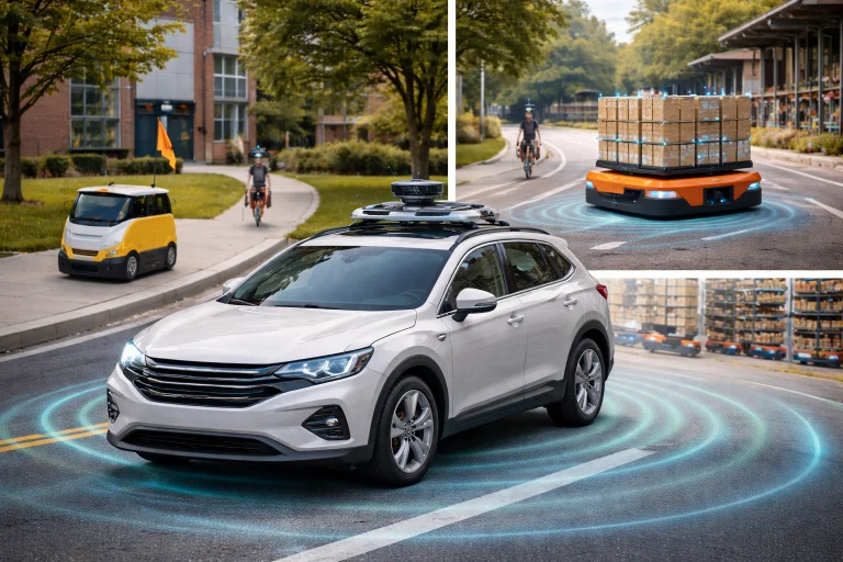
Autonomous Ground Vehicles (AGVs) are mobile robotic systems designed to move safely and intelligently through structured and semi-structured environments such as warehouses, roads, campuses, farms, and industrial facilities. Unlike stationary robots, AGVs must continuously interpret sensor data from LiDAR, cameras, radar, and inertial systems to estimate their position, detect obstacles, and plan safe paths through changing surroundings. Their operation depends on the integration of vehicle kinematics, dynamics, feedback control, and artificial intelligence algorithms that allow them to follow trajectories while maintaining stability and avoiding collisions.
The technologies illustrated reflect the multidisciplinary nature of AGV engineering. Mechanical design provides mobility and traction; sensing systems build a real-time understanding of the environment; planning algorithms generate safe trajectories; and control systems ensure that the vehicle accurately follows those paths. Because AGVs combine perception, computation, and physical motion within a single system, they represent one of the clearest examples of how robotics integrates mathematics, control theory, artificial intelligence, and mechanical engineering into a unified autonomous platform.
Interactive Quick Review: AGV Fundamentals & Integration
Test your understanding of AGV multidisciplinary integration and core mobility systems before exploring kinematic models:
1. What core engineering and scientific domains make up the interdisciplinary nature of Autonomous Ground Vehicles?
Answer: Mechanics, control theory, artificial intelligence, and distributed systems engineering integrated into a unified mobility system.
2. What sensors do AGVs continuously use to estimate position, detect obstacles, and plan safe paths?
Answer: LiDAR, cameras, radar, and inertial measurement units (IMUs).
Kinematic Models of Ground Vehicles
Two commonly used mathematical idealizations describe wheeled mobile robots: the unicycle (differential-drive) model and the bicycle steering model.
Unicycle (Differential-Drive) Model
This model describes the motion of robots whose left and right wheels are driven independently to control both forward velocity and yaw rotation, typical for indoor automated guided vehicles (AGVs) and warehouse autonomous mobile robots (AMRs):
$$\dot{x}(t) = v(t) \cos\theta(t)$$ $$\dot{y}(t) = v(t) \sin\theta(t)$$ $$\dot{\theta}(t) = \omega(t)$$- \(x(t), y(t)\): Planar position coordinates of the robot in the global coordinate frame (\(\text{m}\)).
- \(\theta(t)\): Heading orientation of the vehicle chassis relative to the global \(X\)-axis (\(\text{rad}\)).
- \(v(t)\): Linear forward speed along the vehicle's instantaneous heading vector (\(\text{m/s}\)).
- \(\omega(t)\): Angular turning yaw velocity (\(\text{rad/s}\)).
Bicycle Steering Model
For car-like autonomous vehicles with front-wheel Ackermann steering, the kinematic bicycle model collapses the four wheels into a virtual two-wheel centerline representation:
$$\dot{\theta}(t) = \frac{v(t)}{L} \tan\delta(t)$$- \(L\): Wheelbase distance between the front and rear axles (\(\text{m}\)).
- \(\delta(t)\): Front steering wheel angle relative to the chassis longitudinal centerline (\(\text{rad}\)).
An autonomous research vehicle with wheelbase \(L = 2.50\text{ m}\) travels at longitudinal velocity \(v = 5.0\text{ m/s}\) with front steering angle \(\delta = 8.0^\circ\) (\(0.1396\text{ rad}\)). Calculate the resulting vehicle turning yaw rate \(\dot{\theta}\).
Vehicle Dynamics and Nonlinear Friction Constraints
At higher speeds, kinematic models break down because tire elasticity induces lateral slip angles. Dynamic motion is governed by Newton-Euler kinetics:
$$m a(t) = F_x(t) - F_{\text{drag}}$$Where \(m\) is total vehicle mass, \(a(t)\) is longitudinal acceleration, and \(F_x\) is tire tractive force. Lateral cornering force is physically bounded by the Coulomb-Mohr tire-road friction circle:
$$F_{\text{lat}} \le \mu \cdot m \cdot g$$- \(\mu\): Tire-road friction coefficient (\(0.85\) for dry asphalt; \(0.35\) for wet tarmac; \(0.10\) for ice).
- \(g = 9.81\text{ m/s}^2\): Gravitational acceleration.
An autonomous sedan has mass \(m = 1{,}000\text{ kg}\) operating on a road with friction coefficient \(\mu = 0.70\). Calculate the maximum lateral force the tires can sustain before slipping, and find the maximum cornering speed on a curve of radius \(R = 50.0\text{ m}\).
AGV Technical Challenges and Engineering Solutions
Deploying autonomous ground vehicles across dynamic public highways, mixed industrial factory floors, and unstructured outdoor terrains introduces severe coupled physical and algorithmic constraints. Below are four primary technical challenges and their engineering mitigation frameworks:
The Challenge: Raindrops and airborne fog particles attenuate 905nm LiDAR laser pulses, creating dense backscatter clutter point clouds. Heavy snowfall obscures painted road lane markers, while direct low-angle solar glare blinds CMOS optical camera sensors, leading to catastrophic perception dropouts.
- Imaging Radar & Thermal LWIR Fusion: Fusing high-resolution 4D millimeter-wave radar (77 GHz) and long-wave infrared (LWIR) thermal cameras that penetrate thick atmospheric moisture and smoke independent of visible illumination.
- Dynamic LiDAR Point-Cloud Filtering: Applying spatial-temporal outlier removal and intensity return thresholding to filter out retro-reflective rain droplets and road spray in real time.
- High-Definition (HD) Map Priors: Utilizing centimeter-accurate pre-mapped vector road geometries with localized landmark anchors, allowing the vehicle to track lanes even when surface markings are obscured by snow.
The Challenge: Urban environments are populated by unpredictable human agents, including aggressive drivers, cyclists, and jaywalking pedestrians. Classical constant-velocity motion models fail to predict lane merges, turns, and yielding behaviors, causing "freezing robot" indecision or unsafe trajectory conflicts.
- Spatio-Temporal Graph Neural Networks (ST-GNNs): Modeling interactions between surrounding traffic agents as dynamic graphs where edges encode social compliance, yielding, and spatial proximity.
- Conformal Trajectory Prediction: Generating multi-modal probabilistic trajectory distributions with formal coverage guarantees to account for uncertain human intent.
- Interactive Game-Theoretic Motion Planning: Solving dynamic Stackelberg games online where the autonomous vehicle treats its own maneuvers as active communicative cues to influence surrounding human behavior safely.
The Challenge: Nonlinear Model Predictive Control (NMPC) and real-time obstacle avoidance require solving non-convex constrained quadratic programs (QPs) within strict deadlines (typically \(10\text{–}20\text{ ms}\)). Solver divergence or calculation timeouts at highway speeds can trigger catastrophic trajectory instability.
- Real-Time Iteration (RTI) Schemes: Decoupling optimization into an asynchronous system state linearization phase and a microsecond-level condensed QP feedback phase upon measurement arrival.
- GPU/FPGA-Accelerated Solvers: Implementing custom operator splitting (ADMM) and interior-point algorithms on embedded tensor hardware to guarantee deterministic sub-millisecond execution.
- Warm-Starting via Kinematic Surrogates: Initializing dynamic solvers using low-latency kinematic trajectory solutions from the preceding sampling instant to ensure rapid convergence.
The Challenge: Connected autonomous vehicle fleets rely on Vehicle-to-Everything (V2X) and cellular 5G networks for collaborative intersection crossing and platoon spacing. Wireless links are vulnerable to GPS spoofing, denial-of-service (DoS) jamming, and malicious emergency braking injection.
- IEEE 1609.2 Public Key Infrastructure (PKI): Authenticating every inter-vehicle broadcast packet using hardware security modules (HSM) with microsecond cryptographic signature verification.
- Plausibility Plausibility Checking via Local Sensors: Verifying received V2X telemetry against onboard LiDAR/radar observations before accepting remote guidance commands.
- Autonomous Fallback Mode: Transitioning immediately to an onboard-only safety envelope if V2X packet loss or message corruption is detected.
Path Planning and Trajectory Tracking Control
An AGV tracks a time-parameterized reference trajectory \(\mathbf{x}_r(t) = \begin{bmatrix} x_r(t) & y_r(t) & \theta_r(t) \end{bmatrix}^T\) generated by local lattice or polynomial motion planners. Longitudinal and lateral tracking errors are defined in the Frenét-Serret frame:
$$e_x(t) = x_r(t) - x(t), \quad e_y(t) = y_r(t) - y(t)$$For path tracking, the Stanley Controller computes the front steering command \(\delta(t)\) by combining heading error with a nonlinearly scaled cross-track error term:
$$\delta(t) = (\theta_r - \theta) + \arctan\left(\frac{k \cdot e_y(t)}{v(t)}\right)$$Where \(k\) is a softening tuning gain. At high velocities, the controller smoothly attenuates steering sensitivity to maintain vehicle yaw stability.
Multi-Sensor Fusion and Kalman State Estimation
Accurate state estimation requires fusing complementary data from LiDAR, optical cameras, radar, wheel encoders, and IMUs. The discrete-time Kalman filter update step incorporates fresh observations \(\mathbf{z}_k\) via the optimal gain \(\mathbf{K}_k\):
$$\mathbf{\hat{x}}_k = \mathbf{\hat{x}}_{k|k-1} + \mathbf{K}_k \left(\mathbf{z}_k - \mathbf{H} \mathbf{\hat{x}}_{k|k-1}\right)$$Where \(\mathbf{H}\) is the observation projection matrix. Wheel odometry provides high-frequency relative displacement, while LiDAR-SLAM and RTK-GPS supply drift-free absolute pose corrections.
Fleet Coordination and Spatial Separation
In multi-robot logistics environments, collision-free coordination requires enforcing strict minimum Euclidean spatial separation between any pair of vehicles \(r_i\) and \(r_j\):
$$\|\mathbf{p}_i(t) - \mathbf{p}_j(t)\| \ge d_{\text{safe}}$$Where \(\mathbf{p}_i = \begin{bmatrix} x_i & y_i \end{bmatrix}^T\) and \(d_{\text{safe}}\) includes vehicle physical footprints, turning envelopes, and emergency braking distances.
🎯 Career Guidance Tool Is Autonomous Ground Vehicle Engineering Right For You?Explore autonomous driving engineering pathways, motion planning careers, and mobile robotics system integration. | Explore Career Options → |
Interactive Quick Review: Dynamics, Tracking & Fleet Control
Reinforce key concepts regarding unicycle kinematics, tire friction limits, and fleet collision avoidance before reviewing the FAQ:
1. How does the bicycle steering model capture vehicle geometry differently from the unicycle model?
Answer: The bicycle model accounts for the vehicle's wheelbase (\(L\)) and front-wheel steering angle (\(\delta\)), capturing the non-holonomic Ackermann steering geometry of car-like vehicles.
2. What condition ensures collision-free separation between vehicles in a multi-robot fleet?
Answer: Enforcing that the Euclidean distance between any two vehicle coordinates satisfies \(\|\mathbf{p}_i(t) - \mathbf{p}_j(t)\| \ge d_{\text{safe}}\) for all time \(t\).
External References and Further Reading
To explore advanced research, regulatory frameworks, and industrial developments in autonomous ground vehicles, consult the following authoritative sources:
- NHTSA Automated Vehicles Safety Technologies – Provides official federal guidance, safety frameworks, and regulatory standards for automated driving systems and road testing.
- IEEE Transactions on Intelligent Vehicles – Publishes peer-reviewed research focusing on advanced vehicle control, multi-sensor fusion, motion planning, and intelligent transportation systems.
- SAE International Standard J3016 – Establishes the internationally recognized six-level taxonomy and classification system for motor vehicle automated driving systems.
Frequently Asked Questions about Autonomous Ground Vehicles (AGVs)
What are Autonomous Ground Vehicles, and how do they function?
Autonomous Ground Vehicles (AGVs) are mobile robotic systems that navigate independently across structured or unstructured environments. They operate by continuously capturing multi-sensor data (from LiDAR, cameras, radar, and IMUs) and running real-time SLAM, state estimation, path planning, and feedback control algorithms to steer safely along planned routes.
What is the difference between differential-drive robots and car-like steering AGVs?
Differential-drive robots independently vary the angular velocities of left and right drive wheels, allowing them to spin in place with a zero turning radius. Car-like AGVs use front-wheel Ackermann steering and have a fixed wheelbase, which imposes non-holonomic minimum turning radius constraints modeled by the bicycle kinematic equations.
Why is tire-road friction critical for AGV stability during high-speed turns?
Tire-road friction provides the centripetal lateral force required to alter the vehicle's momentum around curves. If demanded lateral acceleration exceeds available grip (\(F_{\text{lat}} > \mu mg\)), the tire contact patch breaks away, causing understeer, oversteer spin-out, or vehicle rollover.
How do sensor fusion and Kalman filters improve AGV localization?
Single sensors suffer from blind spots: wheel encoders slip, GPS drops in urban canyons, and cameras degrade in glare. Kalman filtering fuses high-rate inertial measurements with absolute landmark observations, statistically balancing noise to yield a smooth, optimal state estimate.
End-of-Page Exercises: Review, Thought-Provoking & Engineering Problems
Section 1: Foundational Review Questions & Answers
1. What are the fundamental equations of the unicycle (differential-drive) kinematic model?
Answer: \(\dot{x}(t) = v(t)\cos\theta(t)\), \(\dot{y}(t) = v(t)\sin\theta(t)\), and \(\dot{\theta}(t) = \omega(t)\).
2. How does the bicycle steering model relate vehicle speed, wheelbase, and steering angle to heading turning rate?
Answer: Through the relationship \(\dot{\theta}(t) = \frac{v(t)}{L} \tan\delta(t)\), where \(L\) is the axle wheelbase and \(\delta\) is the front steering angle.
3. What physical inequality limits the maximum sideways force tires can sustain during cornering without slipping?
Answer: \(F_{\text{lat}} \le \mu mg\), where \(\mu\) is the road-tire friction coefficient, \(m\) is vehicle mass, and \(g\) is gravity.
4. How are path tracking errors defined between a reference planner trajectory and actual vehicle pose?
Answer: By the spatial coordinate differences: \(e_x(t) = x_r(t) - x(t)\) and \(e_y(t) = y_r(t) - y(t)\).
5. What is sensor fusion, and why is it essential for AGV localization?
Answer: Sensor fusion integrates complementary streams (LiDAR, cameras, radar, IMU, wheel encoders) to provide robust, fault-tolerant state estimates that compensate for the individual noise, drift, or environmental vulnerabilities of single sensors.
6. How is propulsion power calculated for an AGV moving at velocity \(v\) with forward traction force \(F_x\)?
Answer: Through the mechanical power formula \(P = F_x \cdot v\).
7. What mathematical condition maintains collision-free separation between vehicles in a multi-robot fleet?
Answer: Enforcing \(\|\mathbf{p}_i(t) - \mathbf{p}_j(t)\| \ge d_{\text{safe}}\) across all vehicle pairs \(i \neq j\) for all time \(t\).
8. What role do Kalman filters play in state estimation update steps?
Answer: They compute an optimal weighting gain (\(\mathbf{K}_k\)) to update a priori model predictions with new noisy observations (\(\mathbf{\hat{x}}_k = \mathbf{\hat{x}}_{k|k-1} + \mathbf{K}_k(\mathbf{z}_k - \mathbf{H}\mathbf{\hat{x}}_{k|k-1})\)).
9. What are common path tracking control methods used in AGV navigation?
Answer: Geometric Pure Pursuit, Stanley steering control, Linear Quadratic Regulators (LQR), and Model Predictive Control (MPC).
10. Why is real-time embedded system design critical for autonomous ground vehicle safety?
Answer: Because braking and steering actuation tasks must execute under hard deterministic timing deadlines to prevent latency-induced instability or catastrophic collisions.
Section 2: Analytical & Thought-Provoking Questions
1. How do unmodeled slippery road surfaces compromise kinematic versus dynamic path tracking?
Answer: Kinematic models assume wheels roll purely without slipping. When black ice or oil violates this assumption, the actual lateral slip angle diverges from zero, rendering kinematic controllers unable to prevent vehicle skidding.
2. What ethical dilemmas emerge when self-driving cars navigate dense pedestrian zones?
Answer: Vehicles must balance progress against over-cautious stopping, weighing passenger comfort against vulnerable road user safety while resolving unpredictable human intentions without eye contact.
3. How does sensor occlusion in heavy traffic impact real-time multi-sensor fusion reliability?
Answer: Large trucks block camera and LiDAR lines of sight, leaving blind spots where the filter must rely on long-range radar reflections and historical spatial track maintenance.
4. What computational bottlenecks occur when executing Model Predictive Control (MPC) on automotive ECUs?
Answer: Long prediction horizons scale the number of decision variables and inequality constraints quadratically, taxing memory bandwidth and compute cycles within strict \(10\text{–}20\text{ ms}\) vehicle control loops.
5. How do nonholonomic constraints restrict an AGV's instantaneous mobility?
Answer: Nonholonomic vehicles cannot translate sideways instantaneously; lateral motion requires coordinating steering angles with forward motion, limiting trajectory agility compared to omnidirectional platforms.
6. What cybersecurity vulnerabilities threaten V2X-connected autonomous fleets?
Answer: Spoofed cooperative awareness messages (CAMs), fake emergency deceleration warnings, or GPS timing attacks can induce phantom braking waves or deliberate intersection pileups.
7. How can reinforcement learning policies trained in simulation be safely transferred to real vehicles?
Answer: Via aggressive domain randomization of tire friction and lighting, combined with deterministic Control Barrier Functions (CBFs) that override neural outputs if safety boundaries are approached.
8. What trade-offs exist between centralized cloud fleet management and decentralized edge coordination?
Answer: Centralized cloud planning produces globally optimal traffic flows but suffers from single points of failure and latency, whereas decentralized edge coordination is resilient but can cause gridlocks at intersections.
9. How do dynamic obstacles challenge standard reactive planners like Artificial Potential Fields?
Answer: Potential fields treat obstacles as static repulsive potentials, which can trap vehicles in local minima or cause unstable oscillations when moving obstacles cross trajectories at speed.
10. What limitations affect camera-based lane detection under extreme solar glare?
Answer: Direct sun glare saturates CMOS pixels, destroying local contrast and causing deep neural networks to drop faint road markings, requiring backup guidance from LiDAR and HD maps.
11. How does vehicle suspension dynamics influence tire contact forces during cornering?
Answer: Road roughness excites vertical suspension modes, causing transient normal force variations that intermittently reduce lateral grip and trigger active electronic stability interventions.
12. What legal frameworks govern liability in autonomous vehicle collisions?
Answer: Liability is apportioned between the human supervisor and system manufacturers (OEM, software developer, sensor vendor) by auditing event data recorders (EDR) against the defined Operational Design Domain (ODD).
Section 3: Numerical Engineering Problems & Solutions
A car-like autonomous ground vehicle has a wheelbase of \(L = 3.0\text{ meters}\) and travels at a constant forward speed of \(v = 12.0\text{ m/s}\). If the front steering angle is set to \(\delta = 10.0^\circ\) (where \(\tan(10.0^\circ) \approx 0.1763\)), calculate the vehicle's heading turning rate \(\dot{\theta}\) in \(\text{rad/s}\).
Bicycle steering model formula: $$\dot{\theta} = \frac{v}{L} \tan\delta$$ Substitute numerical values: $$\dot{\theta} = \frac{12.0\text{ m/s}}{3.0\text{ m}} \times 0.1763 = 4.0 \times 0.1763 = 0.7052\text{ rad/s}$$ Final Answer: Vehicle turning rate is approximately \(0.71\text{ rad/s}\).
An AGV with a total mass of \(m = 1{,}400.0\text{ kg}\) negotiates a curve on dry asphalt where the tire-road friction coefficient is \(\mu = 0.85\). Assuming standard gravitational acceleration \(g = 9.81\text{ m/s}^2\), calculate the maximum allowable lateral cornering force \(F_{\text{lat}}\) before tire slip occurs.
Lateral force limit formula: $$F_{\text{lat}} \le \mu \cdot m \cdot g$$ Substitute numerical values: $$F_{\text{lat}} \le 0.85 \times 1{,}400.0\text{ kg} \times 9.81\text{ m/s}^2$$ $$F_{\text{lat}} \le 0.85 \times 13{,}734.0\text{ N} = 11{,}673.9\text{ N}$$ Final Answer: Maximum allowable lateral cornering force is \(11{,}673.9\text{ N}\).
A heavy industrial AGV generates a forward traction force of \(F_x = 2{,}200.0\text{ N}\) while cruising at a constant longitudinal velocity of \(v = 4.50\text{ m/s}\). Calculate the required mechanical propulsion power \(P\) in Watts and Kilowatts.
Mechanical power formula: $$P = F_x \cdot v$$ Substitute values: $$P = 2{,}200.0\text{ N} \times 4.50\text{ m/s} = 9{,}900.0\text{ Watts}$$ Convert to Kilowatts: $$P_{\text{kW}} = \frac{9{,}900.0\text{ W}}{1{,}000} = 9.90\text{ kW}$$ Final Answer: Required mechanical propulsion power is \(9{,}900\text{ W}\) (\(9.90\text{ kW}\)).
Two warehouse AGVs operate in the same aisle. AGV 1 is located at position coordinates \(\mathbf{p}_1 = \begin{bmatrix} 12.4 & 5.1 \end{bmatrix}^T\text{ meters}\), and AGV 2 is located at position \(\mathbf{p}_2 = \begin{bmatrix} 15.1 & 8.6 \end{bmatrix}^T\text{ meters}\). Calculate the Euclidean distance between the two vehicles and determine if they violate a minimum safe separation distance of \(d_{\text{safe}} = 4.0\text{ meters}\).
Euclidean distance formula: $$d = \|\mathbf{p}_1 - \mathbf{p}_2\| = \sqrt{(x_2 - x_1)^2 + (y_2 - y_1)^2}$$ Compute coordinate differences: $$\Delta x = 15.1 - 12.4 = 2.7\text{ m}, \quad \Delta y = 8.6 - 5.1 = 3.5\text{ m}$$ Sum of squares: $$(\Delta x)^2 + (\Delta y)^2 = (2.7)^2 + (3.5)^2 = 7.29 + 12.25 = 19.54\text{ m}^2$$ Compute square root: $$d = \sqrt{19.54} \approx 4.4204\text{ meters}$$ Compare against threshold: $$d = 4.42\text{ m} \ge d_{\text{safe}} = 4.0\text{ m} \quad (\text{Safe; no violation})$$ Final Answer: Distance between vehicles is \(4.42\text{ meters}\), satisfying safe separation.
An AGV state estimator predicts a longitudinal position of \(\hat{x}_{k|k-1} = 25.0\text{ meters}\). A wheel encoder and GPS sensor fusion measurement reads \(z_k = 25.60\text{ meters}\). If the Kalman gain is set to \(K_k = 0.40\) (with observation matrix \(H = 1\)), calculate the updated posterior state estimate \(\hat{x}_{k|k}\).
Kalman update equation: $$\hat{x}_{k|k} = \hat{x}_{k|k-1} + K_k (z_k - H \hat{x}_{k|k-1})$$ Compute innovation residual: $$\tilde{y}_k = 25.60\text{ m} - (1 \times 25.0\text{ m}) = 0.60\text{ meters}$$ Apply correction: $$\hat{x}_{k|k} = 25.0 + (0.40 \times 0.60) = 25.0 + 0.24 = 25.24\text{ meters}$$ Final Answer: Updated posterior position estimate is \(25.24\text{ meters}\).
An autonomous delivery rover has a total mass of \(m = 250.0\text{ kg}\). If the vehicle's onboard electric powertrain delivers a net driving force of \(F_x = 375.0\text{ N}\) to the wheels, calculate the resulting longitudinal acceleration \(a(t)\) in \(\text{m/s}^2\).
Newton's second law: $$a = \frac{F_x}{m}$$ Substitute numerical values: $$a = \frac{375.0\text{ N}}{250.0\text{ kg}} = 1.50\text{ m/s}^2$$ Final Answer: Resulting longitudinal acceleration is \(1.50\text{ m/s}^2\).
A differential-drive AGV moves with forward linear velocity \(v = 2.0\text{ m/s}\) and heading orientation \(\theta = 30.0^\circ\) relative to the global reference frame. Calculate the instantaneous velocity components along the global axes (\(\dot{x}\) and \(\dot{y}\)). (Use \(\cos(30.0^\circ) = 0.866\) and \(\sin(30.0^\circ) = 0.500\)).
Unicycle kinematic equations: $$\dot{x} = v \cos\theta = 2.0\text{ m/s} \times 0.866 = 1.732\text{ m/s}$$ $$\dot{y} = v \sin\theta = 2.0\text{ m/s} \times 0.500 = 1.000\text{ m/s}$$ Final Answer: Velocity components are \(\dot{x} \approx 1.73\text{ m/s}\) and \(\dot{y} = 1.00\text{ m/s}\).
An electric warehouse AGV draws an average electrical power of \(P = 3.50\text{ kW}\) while transporting goods across a facility for a duration of \(T = 45.0\text{ minutes}\) (\(0.75\text{ hours}\)). Calculate the total electrical energy consumed in kilowatt-hours (\(\text{kWh}\)).
Energy consumption formula: $$E = P \cdot T = 3.50\text{ kW} \times 0.75\text{ h} = 2.625\text{ kWh}$$ Final Answer: Total energy consumed is \(2.625\text{ kWh}\).
An autonomous truck measures a lateral tracking error of \(e_y = 0.45\text{ meters}\) relative to its reference path planner trajectory. If a proportional tracking controller applies a correction steering response gain of \(K_p = 1.20\text{ rad/m}\), calculate the resulting steering command value \(\delta\).
Proportional steering correction law: $$\delta = K_p \cdot e_y = 1.20\text{ rad/m} \times 0.45\text{ m} = 0.540\text{ rad}$$ Convert to degrees: $$\delta_{\text{deg}} = 0.540\text{ rad} \times \left(\frac{180^\circ}{\pi}\right) \approx 0.540 \times 57.2958 \approx 30.94^\circ$$ Final Answer: Commanded steering adjustment is \(0.54\text{ rad}\) (\(\approx 30.94^\circ\)).
An autonomous vehicle LiDAR sensor emits \(250{,}000\text{ points/s}\). Each point transmits 3D spatial coordinates \((x, y, z)\) encoded as 32-bit floating-point values plus a 16-bit reflectivity intensity value. Calculate the raw telemetry data generation rate in Megabits per second (Mbps).
Bits per LiDAR point: $$b_{\text{point}} = (3 \times 32\text{ bits}) + 16\text{ bits} = 96 + 16 = 112\text{ bits/point}$$ Total bit generation rate: $$\text{Rate}_{\text{bps}} = 250{,}000\text{ points/s} \times 112\text{ bits/point} = 28{,}000{,}000\text{ bits/s}$$ Convert to Megabits per second: $$\text{Rate}_{\text{Mbps}} = \frac{28{,}000{,}000\text{ bps}}{10^6} = 28.0\text{ Mbps}$$ Final Answer: LiDAR raw telemetry throughput is \(28.0\text{ Mbps}\).
An autonomous ground vehicle cruises at a forward speed of \(v = 20.0\text{ m/s}\). Upon detecting an obstruction, the perception-to-actuation system reaction latency is \(t_{\text{react}} = 0.30\text{ seconds}\), and the vehicle's emergency braking deceleration rate is constant at \(a = 5.0\text{ m/s}^2\). Calculate the total stopping distance.
Reaction distance: $$d_{\text{react}} = v \cdot t_{\text{react}} = 20.0\text{ m/s} \times 0.30\text{ s} = 6.0\text{ meters}$$ Braking distance (from \(v^2 = 2ad_{\text{brake}}\)): $$d_{\text{brake}} = \frac{v^2}{2a} = \frac{(20.0\text{ m/s})^2}{2 \times 5.0\text{ m/s}^2} = \frac{400.0}{10.0} = 40.0\text{ meters}$$ Total stopping distance: $$d_{\text{total}} = d_{\text{react}} + d_{\text{brake}} = 6.0\text{ m} + 40.0\text{ m} = 46.0\text{ meters}$$ Final Answer: Total vehicle stopping distance is \(46.0\text{ meters}\).
An AGV's safety-critical embedded ECU manages a periodic obstacle-detection task with worst-case execution time \(C = 1.50\text{ ms}\) and repetition period \(T = 10.0\text{ ms}\). Calculate the processor utilization factor \(U\) for this task and determine if it meets standard single-task capacity limits.
Processor utilization formula: $$U = \frac{C}{T} = \frac{1.50\text{ ms}}{10.0\text{ ms}} = 0.150 \Rightarrow 15.0\%$$ Compare against capacity limit: $$U = 0.15 \le 1.0 \quad (\text{Schedulable})$$ Final Answer: Task CPU utilization is \(15.0\%\), well within real-time scheduling boundaries.
Autonomous Ground Vehicles (AGVs) — Summary & Wrap-Up
Autonomous Ground Vehicles integrate mechanical design, kinematic modeling, nonlinear dynamics, multi-sensor fusion, and distributed intelligence into a complete mobility system. By mastering unicycle and bicycle steering models, tire-friction constraints, path tracking control, Kalman filtering, and fleet coordination, AGV engineers build robust autonomous platforms that transform transportation, industrial logistics, agriculture, and service industries.
Autonomous Mobility Within the Robotics Ecosystem
Autonomous ground vehicles represent one of the most visible forms of modern robotics, combining sensing technologies, navigation algorithms, and intelligent control systems to allow machines to move independently through complex environments. While mobility is central to this field, it is closely connected with many other branches of applied robotics that address how robots interact with people, infrastructure, and operational environments.
Safe and effective interaction between humans and autonomous machines is studied in Human–Robot Interaction and Ethics, where topics such as trust, safety frameworks, and interface design shape how autonomous systems operate in public spaces. In industrial environments, mobile robots frequently work alongside stationary automation platforms, a topic explored in Industrial Robotics Systems and Cobots.
Robotics technologies also extend far beyond transportation. For example, precision automation in healthcare is discussed in Medical and Surgical Robotics, while autonomous machines designed for hospitality, assistance, and everyday environments are examined in Service Robotics.
Mobile robotic technologies have also transformed agriculture and logistics. Autonomous sensing and field operations are introduced in Agricultural Robotics, while warehouse automation and coordinated fleets of mobile platforms are explored in Warehouse Logistics and Autonomous Mobile Robots (AMRs).
Ground vehicles represent only one form of robotic mobility. Autonomous flight platforms are discussed in Aerial Robotics and UAV Systems, where navigation, sensing, and mission planning extend robotics into aerial environments.
Readers interested in the broader scientific and engineering principles behind these technologies—including robot perception, control, and intelligent decision-making—can explore the Robotics Hub, which connects the many applied domains of robotics into a unified interdisciplinary field.