
Agricultural robotics addresses the growing need for precision farming, labor efficiency, and sustainable food production. Unlike structured industrial environments, agricultural robots operate in dynamic outdoor settings where terrain irregularities, weather variability, crop growth patterns, and biological uncertainty introduce significant complexity.
These systems must integrate perception, navigation, manipulation, and control in environments that are only partially predictable. Agricultural robotics therefore combines mechanical engineering, sensing technology, artificial intelligence, and control systems into a unified field platform.
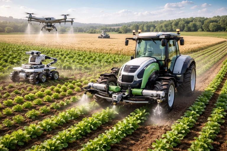
This multi-agent agricultural system demonstrates collaborative field robotics in modern precision farming. An autonomous tractor executes precision tillage and seeding guided by centimeter-level RTK-GPS, while an autonomous ground rover navigates narrow crop rows for targeted weed removal and micro-spraying. Overhead, a multispectral UAV surveys crop canopy health, feeding real-time NDVI indices into the farm management system to dynamically optimize water and nutrient allocation.
Interactive Quick Review: Agricultural Robotics Foundations
Test your understanding of unstructured outdoor challenges and precision farming objectives before exploring modeling equations:
1. How do unstructured agricultural environments differ fundamentally from structured industrial factory settings?
Answer: Agricultural settings are dynamic outdoor spaces where terrain irregularities, weather variability, biological uncertainty, and lighting changes introduce significant unpredictability compared to controlled industrial floors.
2. What is the primary operational objective of precision agriculture enabled by robotics?
Answer: To use sensor-driven data collection to optimize farming activities (such as planting, irrigation, and fertilization) at specific localized coordinates rather than treating entire fields uniformly.
Precision Agriculture and Decision Analytics
Precision agriculture uses sensor-driven data collection to optimize farming activities such as planting, irrigation, fertilization, and harvesting. Instead of treating an entire field uniformly, robots and sensing systems allow farmers to manage conditions at specific locations.
Let:
- \(M(x,y)\): Volumetric soil moisture level at spatial field coordinate \((x,y)\) (percentage).
- \(N(x,y)\): Nitrogen/nutrient concentration in the soil at location \((x,y)\) (\(\text{mg/kg}\)).
- \(H(x,y)\): Plant health index estimated from multispectral imagery (e.g., Normalized Difference Vegetation Index, NDVI).
- \(M_{\text{threshold}}\): Minimum acceptable moisture level required for healthy crop growth.
A deterministic localized irrigation decision rule is modeled as:
$$M(x,y) < M_{\text{threshold}}$$At spatial coordinate \((x_1, y_1)\), an in-situ capacitive sensor measures soil moisture \(M(x_1, y_1) = 18\%\). Agronomic thresholds require \(M_{\text{threshold}} = 22\%\). If a 1.0-hectare field exhibits moisture deficits across only \(30\%\) of its surveyed grid cells, calculate the volumetric water reduction achieved via robotic micro-irrigation versus uniform blanket application (\(40{,}000\text{ L/ha}\)).
Perception in Natural Environments
Agricultural robots must interpret visual, spectral, and geometric sensor data to differentiate cash crops from invasive weed species, detect plant pathogen lesions, and evaluate fruit ripeness under uncontrolled solar illumination.
Let \(\mathbf{I}(x,y)\) denote image intensity at pixel coordinate \((x,y)\), and \(\mathbf{f}(\mathbf{I}) \in \mathbb{R}^d\) represent a high-dimensional feature embedding extracted via a convolutional neural network (CNN) or vision transformer. The maximum a posteriori (MAP) semantic segmentation classification rule is:
$$c^* = \arg\max_{k \in \mathcal{K}} P(k \mid \mathbf{f}(\mathbf{I}))$$Where \(\mathcal{K} = \{\text{crop}, \text{weed}, \text{soil}, \text{obstacle}\}\). Perception pipelines fuse visible RGB channels with Near-Infrared (NIR) bands to calculate reflectance indices such as the Normalized Difference Vegetation Index (NDVI):
$$\text{NDVI} = \frac{\rho_{\text{NIR}} - \rho_{\text{Red}}}{\rho_{\text{NIR}} + \rho_{\text{Red}}}$$Healthy photosynthetic vegetation strongly absorbs red light (\(\approx 660\text{ nm}\)) and strongly reflects near-infrared radiation (\(\approx 840\text{ nm}\)), allowing classifiers to separate living biomass from background soil and non-photosynthetic debris.
Autonomous Field Navigation and Terramechanics
Mobile agricultural rovers typically employ differential drive or Ackermann steering kinematics to navigate narrow crop rows without damaging plant root systems. The planar kinematic equations of motion are:
$$\dot{x} = v \cos\theta, \quad \dot{y} = v \sin\theta, \quad \dot{\theta} = \omega$$Where \(v\) is forward linear velocity, \(\theta\) is heading angle relative to the field datum, and \(\omega\) is yaw turn rate. Because agricultural terrain consists of deformable, cohesive, or saturated topsoil, wheel traction is strictly governed by Coulomb-Mohr terramechanics:
$$F_{\text{traction}} \le \mu \cdot m \cdot g$$- \(\mu\): Effective soil-tire friction/shear coefficient (typically \(0.20\)–\(0.40\) for damp loam; \(0.60\) for dry compacted dirt).
- \(m\): Gross operating mass of the agricultural robot (\(\text{kg}\)).
- \(g = 9.81\text{ m/s}^2\): Gravitational acceleration.
An autonomous field rover with total mass \(m = 800\text{ kg}\) operates on damp clay soil where the traction coefficient is \(\mu = 0.50\). Calculate the maximum tractive force before longitudinal wheel slip occurs, and compute the maximum allowable linear acceleration \(a_{\max}\).
Agricultural Robotics Challenges and Engineering Solutions
Deploying autonomous robotic hardware in uncontrolled agronomic environments presents severe operational bottlenecks. Below are four primary technical challenges and their engineering mitigation frameworks:
The Challenge: Crops grow irregularly, change morphology dynamically over the season, and overlap heavily within dense foliage. Ripening fruit is frequently occluded by leaves and branches. Furthermore, outdoor lighting shifts constantly from direct sun glare to deep leaf shadows, causing conventional RGB segmentation models to fail.
- Active Perception and Multi-View Visual Servoing: Robotic arms dynamically adjust end-effector camera viewpoints around canopy clusters, generating dense 3D point clouds to mathematically reconstruct obscured crop geometries.
- Multispectral and Hyperspectral Imaging: Integrating narrow-band sensors that isolate chlorophyll and water absorption bands, rendering crop classification invariant to ambient visible light variations.
- Deep Synthetic Data Augmentation: Training semantic neural networks using domain-randomized 3D synthetic plant models generated in physics simulators to bridge the sim-to-real gap across diverse weather conditions.
The Challenge: Agricultural soils vary from loose sand to heavy, waterlogged clay. Saturated soils cause tire sinkage and wheel slip ratios exceeding \(40\%\), which invalidates standard wheel odometry and can lead to rovers becoming hopelessly stuck in the field.
- Terramechanics Slip Observers: Executing real-time Bekker-Wong soil mechanics observers in the drive inverter, comparing wheel angular velocity with Doppler radar or optical ground speed sensors to modulate individual wheel torque before slip occurs.
- Independent All-Wheel Steer and Drive (4WD/4WS): Utilizing independent in-hub brushless motors and articulated steering knuckles to execute crabbing maneuvers and zero-radius turns without scrubbing soil.
- Continuous Rubber Track Modules: Replacing pneumatic tires with wide continuous rubber crawler tracks to lower ground contact pressure below \(20\text{ kPa}\), preventing subsurface soil compaction.
The Challenge: Agricultural implements operate in thick abrasive dust, corrosive chemical spray mists, torrential rains, and direct solar heating up to \(45^\circ\text{C}\). Dust coats optical lenses, chemical sprays corrode connectors, and persistent low-frequency vibration fatigues solder joints.
- Hermetic IP67/IP69K Enclosures: Packaging electronics and motor controllers into cast aluminum housings rated for high-pressure washdown and steam cleaning.
- Active Sensor Cleaning Systems: Equipping optical cameras and LiDAR covers with compressed-air blast nozzles and hydrophobic coatings that periodically purge dust and dew.
- Conductive and Phase-Change Thermal Pathways: Routing thermal dissipation from internal compute units directly to the heavy metal chassis via heat pipes, eliminating failure-prone external cooling fans.
The Challenge: Field operations require high sustained power: a heavy weeding or tilling implement can consume tens of kilowatts. Pure battery-electric platforms face severe runtime constraints, requiring frequent recharging that interrupts time-critical planting and harvesting windows.
- Decentralized Swarm Architecture: Replacing single massive multi-ton tractors with cooperating fleets of lightweight (\(< 100\text{ kg}\)) battery-powered rovers operating continuously in parallel.
- Autonomous Mobile Docking & Battery Swapping: Designing autonomous perimeter stations where field rovers dock and exchange depleted battery packs in under three minutes without human intervention.
- Solar-Electric Supplemental Arrays: Integrating wide monocrystalline photovoltaic canopies on the rover roof to trickle-charge batteries during operation, extending daily runtimes by \(20\text{–}35\%\).
Energy Efficiency and Electrical Power Budgeting
Agricultural robots must operate across large acreages for extended shifts, making electrical energy management critical. Cumulative energy expenditure over an operational window \([0, T]\) is:
$$E = \int_0^T P(t) \, dt$$Where \(P(t) = P_{\text{drive}}(t) + P_{\text{implement}}(t) + P_{\text{compute}}(t)\) reflects the summed instantaneous power of traction motors, active weeding tools (lasers, mechanical cultivators, spray pumps), and embedded GPU computers.
An autonomous weeding rover operates with an average continuous power draw of \(P = 2.50\text{ kW}\) across an uninterrupted field shift of \(T = 6.0\text{ hours}\). Calculate total electrical energy consumed in kilowatt-hours (\(\text{kWh}\)) and Megajoules (\(\text{MJ}\)).
Case Study: Autonomous Tractor Row-Following Control
Autonomous tractors track crop rows using RTK-GPS and forward-looking vision/LiDAR systems. Let \(y_d(t)\) denote the planned crop row centerline coordinate and \(y(t)\) represent the measured lateral position of the vehicle centerline. The lateral tracking error is:
$$e(t) = y_d(t) - y(t)$$Applying a proportional-derivative (PD) steering control law to adjust the front wheel steering angle \(\delta(t)\):
$$\delta(t) = K_P e(t) + K_D \dot{e}(t)$$An autonomous tractor traveling down a corn row detects a lateral deviation of \(e = 0.15\text{ m}\). The onboard steering controller operates with proportional gain \(K = 0.80\text{ rad/m}\). Calculate the commanded steering angle adjustment \(\delta\) in radians and convert to degrees.
Yield Modeling and Predictive Agronomic Analytics
Agricultural robots continuously log georeferenced sensor layers during field passes, providing spatial inputs to predict localized harvest yield \(Y(x,y)\) (metric tons per hectare):
$$Y(x,y) = f(H(x,y), N(x,y), M(x,y))$$Where \(H\) is plant canopy vigor, \(N\) is soil nitrate availability, and \(M\) is volumetric moisture. Linearized empirical models relate these parameters to evaluate spatial yield variance:
$$Y(x,y) = \beta_0 + \beta_1 H(x,y) + \beta_2 N(x,y) + \beta_3 M(x,y)$$Farmers utilize these predictive heatmaps to forecast total harvest volumes, pre-book grain storage facilities, and optimize harvesting logistics weeks in advance.
🎯 Career Guidance Tool Is Agricultural Robotics & Precision Farming Right For You?Explore field robotics engineering pathways, agronomic AI careers, and autonomous agricultural machinery design. | Explore Career Options → |
Interactive Quick Review: Perception, Navigation & Sustainability
Reinforce key concepts regarding field perception classification, traction constraints, and environmental impacts before reviewing the FAQ:
1. How do perception algorithms classify elements like crops versus weeds in natural farm settings?
Answer: By extracting feature vectors (color, shape, texture, multispectral reflectance) from image data and assigning predicted class labels based on maximum probability evaluation (\(c = \arg\max_{k} P(k \mid \mathbf{f}(\mathbf{I}))\)).
2. What environmental benefit is achieved by targeted micro-spraying compared to uniform chemical application?
Answer: Targeted spraying drastically reduces chemical quantities (\(Q_{\text{targeted}} < Q_{\text{uniform}}\)), minimizing harmful chemical runoff into surrounding watersheds and reducing herbicide build-up in the soil.
Frequently Asked Questions about Agricultural Robotics
What is agricultural robotics, and why is it transforming modern farming?
Agricultural robotics is the deployment of autonomous cyber-physical machines, artificial intelligence, and mechatronic implements to farm management. It transforms food production by mitigating farm labor shortages, reducing agricultural chemical consumption by up to \(90\%\), conserving water, and increasing per-hectare yield through plant-level management.
How do field robots handle soft, uneven, or muddy soil conditions?
Field robots utilize terramechanic models that predict wheel slip based on the soil-tire friction coefficient (\(\mu\)). Drive controllers use independent all-wheel speed monitoring and slip observers to modulate motor torques dynamically, preventing wheel spin and vehicle entrapment in saturated ground.
What role does computer vision play in weed control and crop monitoring?
High-speed edge cameras capture live crop row imagery, feeding convolutional neural networks that segment weeds from crop foliage in real time. This triggers localized micro-dose sprayers or high-energy mechanical weeding tools with millimeter precision, eliminating weeds without damaging cash crops.
How do autonomous tractors maintain precise alignment along crop rows?
Autonomous tractors fuse Real-Time Kinematic GPS (RTK-GPS) providing \(\pm 2\text{ cm}\) accuracy with forward-looking LiDAR and vision row-detection pipelines. Feedback controllers continuously compute lateral tracking offsets and adjust electro-hydraulic steering valves to track path centerlines.
End-of-Page Exercises: Review, Thought-Provoking & Engineering Problems
Section 1: Foundational Review Questions & Answers
1. What is the primary operational objective of precision agriculture?
Answer: To optimize farming activities like irrigation and fertilization at specific spatial locations rather than treating entire fields uniformly.
2. How do perception systems classify natural objects like crops, weeds, or soil?
Answer: By extracting image feature vectors and evaluating classification rules to assign the object class with the highest probability (\(c = \arg\max_{k} P(k \mid \mathbf{f}(\mathbf{I}))\)).
3. What kinematic equations describe the planar motion of a wheeled agricultural robot?
Answer: \(\dot{x} = v \cos\theta\), \(\dot{y} = v \sin\theta\), and \(\dot{\theta} = \omega\), relating linear forward velocity and turning rate to global coordinate changes.
4. What physical factor limits the maximum traction force of a mobile robot operating on soft soil?
Answer: The soil-tire shear friction coefficient combined with the normal gravitational force of the robot (\(F_{\text{traction}} \le \mu mg\)).
5. How is total energy consumption calculated for an agricultural robot operating over time interval [0,T]?
Answer: By integrating instantaneous electrical power consumption over total operating duration (\(E = \int_0^T P(t) \, dt\)).
6. What role does feedback control play in autonomous tractor row-following?
Answer: It continuously monitors lateral deviation between the vehicle center and the crop row, applying corrective steering angles proportional to error (\(\delta = Ke\)).
7. How do agricultural robots contribute to crop yield forecasting?
Answer: By logging spatial arrays of canopy health, soil moisture, and nitrogen indices during passes to populate empirical yield models (\(Y(x,y) = f(H, N, M)\)).
8. What environmental advantages do targeted micro-spraying and mechanical weeding provide?
Answer: They drastically reduce pesticide and herbicide application volumes, preventing toxic chemical runoff into groundwaters and curbing soil degradation.
9. What mapping and localization techniques are commonly integrated with GPS for field navigation?
Answer: RTK-GPS is tightly fused with inertial measurement units (IMUs), wheel encoders, and visual-LiDAR SLAM algorithms to maintain navigation during canopy satellite dropouts.
10. Why is mechanical robustness particularly critical for agricultural robots compared to warehouse AMRs?
Answer: Because farm robots face harsh outdoor conditions including abrasive dust, mud, high humidity, chemical sprays, shock loads, and extreme operating temperatures.
Section 2: Analytical & Thought-Provoking Questions
1. How does soil compaction caused by heavy agricultural machinery impact long-term soil ecology?
Answer: Heavy tractors compress soil pores, reducing oxygen availability and rainwater infiltration while restricting root elongation. Lightweight robotic swarms mitigate this damage by distributing field tasks across lighter footprints.
2. What computer vision limitations occur when dense crop canopies obscure ripening fruits?
Answer: Leaves and overlapping branches obscure target produce from standard perspectives, requiring robotic manipulators to deploy eye-in-hand cameras that actively displace foliage and synthesize 3D volumes.
3. How can multi-robot agricultural fleets coordinate task allocation across expansive fields?
Answer: Through decentralized auction algorithms and cellular mesh networking, rovers dynamically bid on unworked field sectors based on battery state-of-charge, tool payload, and proximity.
4. What economic barriers prevent small-scale family farms from adopting advanced agricultural robotics?
Answer: Substantial capital expenditure requirements, limited compatibility with legacy farming implements, and a lack of local servicing technicians for specialized mechatronic subsystems.
5. How does sudden rainfall invalidate pre-computed robot navigation paths?
Answer: Rain rapidly softens soil, decreasing the traction coefficient \(\mu\) and increasing sinkage. Pre-computed paths become impassable, requiring dynamic rerouting to avoid low-lying saturated drainage zones.
6. What legal liabilities arise if an autonomous sprayer damages neighboring organic crops?
Answer: Questions of liability partition between the software navigation provider, the spray controller manufacturer, and the grower, particularly if wind drift sensors failed to halt spraying near parcel borders.
7. How can roof-mounted solar canopies alter the operating economics of field rovers?
Answer: Solar arrays supply auxiliary power for onboard computing and sensor payloads, reducing battery discharge rates and extending daily operational windows during sunny cultivation seasons.
8. What challenges do unstructured weed distributions present for deep learning edge classifiers?
Answer: Early-stage weed seedlings closely mirror emergent cash crops in color and morphology. Classifiers running on low-power edge tensor hardware must perform high-resolution inference within millisecond deadlines.
9. How do variable-rate sprayers dynamically modulate chemical dosing?
Answer: Pulse-width modulation (PWM) solenoid valves open and close at high frequencies, adjusting output volume per millisecond to match real-time weed density maps without changing spray droplet sizes.
10. What engineering trade-offs exist between heavy autonomous tractors and lightweight robot swarms?
Answer: Heavy tractors provide massive pulling force for deep plowing but induce deep soil compaction. Swarms eliminate compaction and offer single-unit failure resilience but require robust wireless networking.
11. How do seasonal crop growth stages alter robotic navigation architectures?
Answer: Emergent crops provide clear ground visual contrast for camera tracking, whereas fully mature crops close canopy lines overhead, blocking GPS signals and requiring 3D LiDAR stem tracking.
12. What cybersecurity risks threaten autonomous tractor fleets?
Answer: Malicious actors can spoof cellular RTK-GPS correction streams or inject false steering commands, driving multi-ton autonomous vehicles off-track and destroying crops or infrastructure.
Section 3: Numerical Engineering Problems & Solutions
A 2.0-hectare agricultural field requires \(40{,}000\text{ liters}\) of water per hectare when irrigated uniformly. Sensor mapping reveals that only \(25\%\) of the field area falls below the moisture threshold requiring water. Calculate the total water volume consumed using targeted precision irrigation and determine the water volume saved.
Total uniform water volume: $$V_{\text{uniform}} = 2.0\text{ ha} \times 40{,}000\text{ L/ha} = 80{,}000\text{ liters}$$ Targeted irrigated area: $$A_{\text{target}} = 2.0\text{ ha} \times 0.25 = 0.50\text{ hectares}$$ Targeted water volume consumed: $$V_{\text{targeted}} = 0.50\text{ ha} \times 40{,}000\text{ L/ha} = 20{,}000\text{ liters}$$ Water volume conserved: $$\Delta V = 80{,}000\text{ L} - 20{,}000\text{ L} = 60{,}000\text{ liters}$$ Final Answer: Targeted irrigation consumes \(20{,}000\text{ L}\), saving \(60{,}000\text{ liters}\) (\(75\%\)).
An agricultural field rover has a total mass of \(m = 650.0\text{ kg}\). Operating on damp clay soil, the soil-tire friction coefficient is measured at \(\mu = 0.35\). Assuming gravitational acceleration \(g = 9.81\text{ m/s}^2\), calculate the maximum allowable traction force before wheel slip occurs.
Traction limit formula: $$F_{\text{traction}} \le \mu \cdot m \cdot g$$ Substitute numerical values: $$F_{\text{traction}} = 0.35 \times 650.0\text{ kg} \times 9.81\text{ m/s}^2$$ $$F_{\text{traction}} = 0.35 \times 6{,}376.5\text{ N} = 2{,}231.775\text{ N}$$ Final Answer: Maximum allowable traction force is approximately \(2{,}231.78\text{ N}\).
An autonomous weeding rover operates with an average electrical power consumption of \(P = 1.80\text{ kW}\) over an uninterrupted field shift of \(T = 7.50\text{ hours}\). Calculate the total energy consumed in kilowatt-hours (\(\text{kWh}\)) and Megajoules (\(\text{MJ}\)). (\(1\text{ kWh} = 3.6\text{ MJ}\)).
Energy consumed in kilowatt-hours: $$E = P \cdot T = 1.80\text{ kW} \times 7.50\text{ h} = 13.50\text{ kWh}$$ Convert to Megajoules: $$E_{\text{MJ}} = 13.50\text{ kWh} \times 3.6\text{ MJ/kWh} = 48.60\text{ MJ}$$ Final Answer: Total energy consumed is \(13.50\text{ kWh}\) (\(48.60\text{ MJ}\)).
An autonomous tractor navigating a crop row detects a lateral tracking error of \(e = 0.22\text{ meters}\). If the controller proportional gain is set to \(K = 0.75\text{ rad/m}\), calculate the required steering angle adjustment \(\delta\) in radians and convert it to degrees.
Proportional steering equation: $$\delta = K \cdot e = 0.75\text{ rad/m} \times 0.22\text{ m} = 0.165\text{ rad}$$ Convert to degrees: $$\delta_{\text{deg}} = 0.165\text{ rad} \times \left(\frac{180^\circ}{\pi}\right) = 0.165 \times 57.29578 \approx 9.4538^\circ$$ Final Answer: Required steering correction is \(0.165\text{ rad}\) (\(9.45^\circ\)).
A farm applies a baseline uniform herbicide spray rate of \(Q_{\text{uniform}} = 12.0\text{ L/ha}\) across a 15.0-hectare field. Utilizing targeted weed-detection robotics, herbicide is applied only to localized weed patches covering \(35\%\) of the total acreage. Calculate the total herbicide volume used and the volume saved.
Total uniform volume: $$V_{\text{uniform}} = 15.0\text{ ha} \times 12.0\text{ L/ha} = 180.0\text{ liters}$$ Targeted spray volume: $$V_{\text{targeted}} = 180.0\text{ L} \times 0.35 = 63.0\text{ liters}$$ Chemical volume saved: $$\Delta V = 180.0\text{ L} - 63.0\text{ L} = 117.0\text{ liters}$$ Final Answer: Targeted spraying consumes \(63.0\text{ L}\), saving \(117.0\text{ liters}\) (\(65\%\)).
An agricultural robot follows a straight crop row with forward chassis speed \(v = 1.25\text{ m/s}\) while maintaining a heading angle \(\theta = 20.0^\circ\) relative to the global reference axis. Calculate the rate of change of position along the \(x\)-axis (\(\dot{x}\)). (Use \(\cos(20.0^\circ) = 0.9397\)).
Planar kinematic equation: $$\dot{x} = v \cos\theta$$ Substitute values: $$\dot{x} = 1.25\text{ m/s} \times 0.9397 = 1.174625\text{ m/s}$$ Final Answer: Rate of change along the \(x\)-axis is approximately \(1.17\text{ m/s}\).
An electric agricultural robot requires a continuous power supply of \(P = 2.0\text{ kW}\) and must operate for a minimum duration of \(T = 5.0\text{ hours}\). If the rover operates on a \(48.0\text{ V}\) nominal DC battery architecture, calculate the required minimum energy capacity in Watt-hours (\(\text{Wh}\)) and Ampere-hours (\(\text{Ah}\)).
Required energy capacity: $$E = P \cdot T = 2{,}000\text{ W} \times 5.0\text{ h} = 10{,}000\text{ Wh} \quad (10.0\text{ kWh})$$ Ampere-hours rating: $$\text{Capacity}_{\text{Ah}} = \frac{E}{V} = \frac{10{,}000\text{ Wh}}{48.0\text{ V}} \approx 208.333\text{ Ah}$$ Final Answer: Minimum battery capacity is \(10{,}000\text{ Wh}\) (\(208.33\text{ Ah}\)).
A predictive corn yield model is given by \(Y(x,y) = 4.0H + 2.5N + 1.8M\), where \(H\) is the plant health index (\(0\) to \(1\)), \(N\) is the soil nutrient index (\(0\) to \(1\)), and \(M\) is the soil moisture index (\(0\) to \(1\)). At a specific field coordinate, sensor measurements yield \(H = 0.80\), \(N = 0.70\), and \(M = 0.90\). Calculate the predicted crop yield \(Y\) in metric tons per hectare.
Evaluate the linear yield model: $$Y = 4.0(0.80) + 2.5(0.70) + 1.8(0.90)$$ $$Y = 3.20 + 1.75 + 1.62 = 6.57\text{ tons/ha}$$ Final Answer: Predicted localized crop yield is \(6.57\text{ metric tons/hectare}\).
A differential-drive agricultural rover moves at forward velocity \(v = 1.50\text{ m/s}\). When executing a row-change headland turn, its angular turning yaw rate is \(\omega = 0.75\text{ rad/s}\). Calculate the instantaneous turning radius \(R\) of the vehicle.
Turning radius relation: $$R = \frac{v}{\omega}$$ Substitute values: $$R = \frac{1.50\text{ m/s}}{0.75\text{ rad/s}} = 2.00\text{ meters}$$ Final Answer: Instantaneous turning radius is \(2.00\text{ meters}\).
An autonomous field mapping rover transmits multispectral imagery and LiDAR point clouds. The multispectral camera captures 15 frames per second at \(2.40\text{ Mb}\) per frame. The LiDAR sensor streams \(200{,}000\text{ points/s}\) with each point encoded as 32 bits (4 bytes). Calculate the total telemetry throughput in Megabits per second (Mbps).
Camera throughput: $$\text{Rate}_{\text{camera}} = 15\text{ fps} \times 2.40\text{ Mb/frame} = 36.0\text{ Mbps}$$ LiDAR throughput: $$\text{Rate}_{\text{LiDAR}} = 200{,}000\text{ points/s} \times 32\text{ bits/point} = 6{,}400{,}000\text{ bps} = 6.40\text{ Mbps}$$ Total telemetry bandwidth: $$\text{Rate}_{\text{total}} = 36.0 + 6.40 = 42.40\text{ Mbps}$$ Final Answer: Combined telemetry bandwidth is \(42.40\text{ Mbps}\).
An agricultural rover of mass \(m = 500.0\text{ kg}\) ascends an inclined orchard slope with grade angle \(\alpha = 12.0^\circ\) at a constant forward speed \(v = 0.80\text{ m/s}\). Assuming \(g = 9.81\text{ m/s}^2\), calculate the mechanical power \(P\) required solely to overcome the rate of gravitational potential energy increase. (Use \(\sin(12.0^\circ) = 0.2079\)).
Gravitational resistance force along slope: $$F_g = m \cdot g \cdot \sin(\alpha) = 500.0\text{ kg} \times 9.81\text{ m/s}^2 \times 0.2079 \approx 1{,}019.75\text{ N}$$ Mechanical climbing power: $$P = F_g \cdot v = 1{,}019.75\text{ N} \times 0.80\text{ m/s} = 815.80\text{ Watts}$$ Final Answer: Required mechanical climbing power is approximately \(815.80\text{ W}\).
A fleet of 4 identical autonomous weeding rovers operates across a soybean farm. Each rover covers an effective field area of \(3.50\text{ hectares/hour}\). If the fleet operates for \(6.0\text{ hours/day}\), calculate the total cumulative crop area serviced by the fleet in one day.
Daily coverage per rover: $$A_1 = 3.50\text{ ha/h} \times 6.0\text{ h} = 21.0\text{ hectares/day}$$ Fleet coverage (4 rovers): $$A_{\text{total}} = 4 \times A_1 = 4 \times 21.0\text{ ha} = 84.0\text{ hectares/day}$$ Final Answer: Total cumulative field area covered is \(84.0\text{ hectares/day}\).
Agricultural Robotics — Summary & Wrap-Up
Agricultural robotics bridges advanced engineering and sustainable food production by deploying intelligent autonomous systems into dynamic outdoor environments. By mastering precision agriculture metrics, natural environment perception, kinematic field navigation, energy optimization, and closed-loop control, agricultural robotics engineers create resilient field machines that conserve vital resources, reduce environmental chemical runoff, and secure global food supplies.
Robotics Technologies Across Agricultural and Environmental Systems
Agricultural robotics applies sensing, automation, and intelligent navigation to large outdoor environments. Autonomous tractors, crop-monitoring drones, and robotic harvesters allow farmers to monitor fields, manage resources efficiently, and respond to environmental conditions in real time. These systems combine perception technologies, mobility platforms, and decision-making algorithms that are shared with many other branches of applied robotics.
For example, aerial monitoring platforms used in crop inspection and environmental surveying are closely related to systems studied in Aerial Robotics and UAV Systems, where autonomous flight control and sensor integration support mapping and surveillance tasks. Ground-based robotic mobility used in field vehicles also shares technological foundations with Autonomous Ground Vehicles, which explore navigation, obstacle detection, and route planning for mobile robotic platforms.
Automation technologies used in agriculture are also connected with industrial robotics. High-precision robotic manipulators and automated production systems operating in factories are introduced in Industrial Robotics Systems and Cobots. Similarly, robotic coordination and material movement in distribution facilities are discussed in Warehouse Logistics and Autonomous Mobile Robots (AMRs), where fleets of mobile robots manage storage and transportation tasks.
Robots designed to interact safely with people are another important area of research. Safety frameworks, ethical design considerations, and communication interfaces between humans and machines are examined in Human–Robot Interaction and Ethics. Related service-oriented robotic platforms supporting hospitality, healthcare assistance, and public environments are explored in Service Robotics.
Robotics technologies also contribute to advanced medical procedures through precision instruments and teleoperated surgical systems. These applications are discussed in Medical and Surgical Robotics, demonstrating how robotics continues to expand across diverse sectors of modern technology.
Students who wish to understand the broader scientific and engineering principles behind these applications—including robot perception, motion planning, and intelligent control systems—can explore the Robotics Hub, which introduces the interdisciplinary foundations that connect these applied robotics domains.