
Maxwell’s equations are the central laws of classical electrodynamics. They explain how electric fields, magnetic fields, electric charge, electric current, and changing fields are connected. Together with the Lorentz force law, they form the foundation for understanding electric circuits, electromagnetic induction, electromagnetic waves, antennas, optical systems, radiation pressure, and many modern technologies.
At first, the four equations may look like a compact set of mathematical statements. Their physical meaning is much richer. One equation tells us how electric charge produces electric field. Another tells us that isolated magnetic poles have not been observed in classical electromagnetism. A third tells us that changing magnetic fields produce circulating electric fields. The fourth, completed by Maxwell, tells us that electric currents and changing electric fields produce magnetic fields.
The great power of Maxwell’s equations is that they turn many separate facts about electricity and magnetism into one coherent field theory. They show that electric and magnetic effects are not separate worlds, but two connected aspects of one electromagnetic system.
For students preparing for university physics or engineering, Maxwell’s equations in electrodynamics are a gateway. They link electrostatics, circuits, magnetostatics, induction, electromagnetic waves, energy flow, relativity, optics, and communication technology into a single framework.
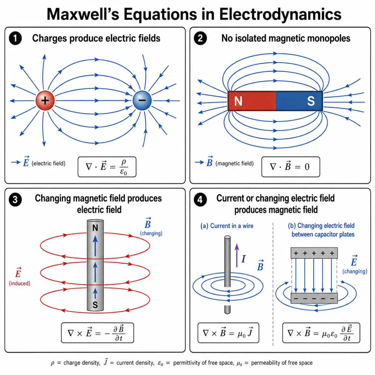
This illustration presents Maxwell’s equations in electrodynamics as four connected field laws. The first panel shows electric field lines spreading outward from a positive charge and inward toward a negative charge. The second panel shows magnetic field lines forming closed loops around a bar magnet, illustrating that there are no isolated magnetic monopoles. The third panel shows a changing magnetic field producing an induced electric field. The fourth panel shows how an electric current, or a changing electric field between capacitor plates, produces a magnetic field. The picture helps students see Maxwell’s equations as a compact map of how electric and magnetic phenomena shape one another.
Learning Pathway
This page belongs to the Electrodynamics cluster under Electricity and Magnetism. It introduces Maxwell’s equations as the central field laws, then connects them to charge conservation, energy flow, electromagnetic waves, and relativity.
Electricity and Magnetism
Start from the wider field of electric charge, electric fields, magnetic fields, circuits, induction, and electromagnetic interactions.Electrodynamics
Study electric and magnetic fields when they change with time, interact with charges and currents, and carry energy through space.Maxwell’s Equations in Electrodynamics
Understand the four field laws that organise classical electromagnetism into one unified theory.Charge Conservation and Continuity
Learn why electric charge cannot simply disappear, and how current density and the continuity equation express local charge conservation.Electromagnetic Energy and Poynting Vector
Explore how electromagnetic fields store energy, transfer power, and send energy flow through space using the Poynting vector.Relativity and Electromagnetism
See how electric and magnetic fields are linked by motion, reference frames, and special relativity.Structural Hierarchy
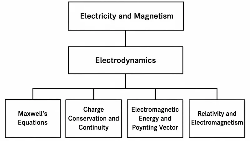
This structural hierarchy chart shows the Electrodynamics cluster within the wider Electricity and Magnetism section. Electricity and Magnetism appears at the top as the parent area, followed by Electrodynamics as the cluster hub. Below Electrodynamics are four child pages: Maxwell’s Equations, Charge Conservation and Continuity, Electromagnetic Energy and Poynting Vector, and Relativity and Electromagnetism. The chart helps students see how Maxwell’s Equations provides the field-law foundation for the rest of the Electrodynamics pathway.
What Maxwell’s Equations in Electrodynamics Really Mean
Maxwell’s equations describe fields, not only forces. This distinction is important. A force tells us what happens to a particular charge. A field describes what exists in space and time, even before a test charge is placed there.
The electric field tells us how a charge would be pushed or pulled. The magnetic field tells us how moving charges or currents would be affected. Maxwell’s equations tell us where these fields come from, how they spread, how they curl, and how they change with time.
In electrostatics, charges produce electric fields. In magnetostatics, currents produce magnetic fields. In electrodynamics, fields can change with time, and changing fields can produce other fields. This dynamic field behaviour is what makes electromagnetic waves possible.
The Four Equations at a Glance
Gauss’s Law for Electricity
Electric charge is the source or sink of electric field. Positive charge sends electric field outward, while negative charge draws electric field inward.Gauss’s Law for Magnetism
Magnetic field lines do not begin or end at isolated magnetic charges. Instead, magnetic field lines form closed loops in classical electromagnetism.Faraday’s Law of Induction
A changing magnetic field produces a circulating electric field. This principle supports generators, transformers, induction coils, and many electrical technologies.Ampère–Maxwell Law
Electric current and changing electric field produce magnetic field. Maxwell’s added displacement current term made the theory complete and predicted electromagnetic waves.Maxwell’s Equations in Differential Form
The differential form describes what happens locally, at each point in space. It is especially useful in university electrodynamics because it reveals how fields behave point by point.
Gauss’s law for electricity:
\( \nabla \cdot \vec{E} = \frac{\rho}{\varepsilon_0} \)
This equation says that electric charge density \( \rho \) acts as a local source of electric field divergence. Where there is positive charge, electric field tends to spread outward. Where there is negative charge, electric field tends to converge inward.
Gauss’s law for magnetism:
\( \nabla \cdot \vec{B} = 0 \)
This equation says that magnetic field has no ordinary source or sink in classical electromagnetism. Magnetic field lines do not begin or end at isolated north or south magnetic charges.
Faraday’s law of induction:
\( \nabla \times \vec{E} = -\frac{\partial \vec{B}}{\partial t} \)
This equation says that a changing magnetic field produces a curling electric field. The minus sign expresses Lenz’s law: the induced effect opposes the change that produces it.
Ampère–Maxwell law:
\( \nabla \times \vec{B} = \mu_0\vec{J} + \mu_0\varepsilon_0\frac{\partial \vec{E}}{\partial t} \)
This equation says that magnetic field can curl around electric current density \( \vec{J} \), and also around a changing electric field. The second term, \( \mu_0\varepsilon_0\frac{\partial \vec{E}}{\partial t} \), is Maxwell’s displacement current contribution.
Pictorial Illustration 1: The Four Local Field Laws
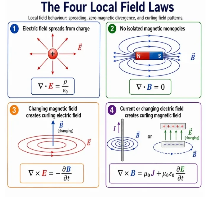
This illustration presents the four local field laws of Maxwell’s equations in electrodynamics. The first panel shows electric field lines spreading outward from electric charge. The second panel shows magnetic field lines forming closed loops, indicating that isolated magnetic monopoles are not found in classical electromagnetism. The third panel shows a changing magnetic field producing a curling electric field. The fourth panel shows that electric current, or a changing electric field, can produce a curling magnetic field. The picture helps students understand the differential form of Maxwell’s equations as a local description of how electric and magnetic fields behave at each point in space.
Maxwell’s Equations in Integral Form
The integral form describes field behaviour over extended surfaces and paths. It is especially useful when dealing with symmetry, flux, circulation, enclosed charge, and total current through a surface.
Gauss’s law for electricity:
\( \oint \vec{E} \cdot d\vec{A} = \frac{Q_{\text{enc}}}{\varepsilon_0} \)
The total electric flux through a closed surface depends on the net charge enclosed by that surface.
Gauss’s law for magnetism:
\( \oint \vec{B} \cdot d\vec{A} = 0 \)
The total magnetic flux through a closed surface is zero. Magnetic field lines entering a closed surface must also leave it.
Faraday’s law of induction:
\( \oint \vec{E} \cdot d\vec{l} = -\frac{d\Phi_B}{dt} \)
A changing magnetic flux produces an induced electric circulation around a loop.
Ampère–Maxwell law:
\( \oint \vec{B} \cdot d\vec{l} = \mu_0 I_{\text{enc}} + \mu_0\varepsilon_0\frac{d\Phi_E}{dt} \)
Magnetic circulation around a path depends on the enclosed conduction current and the rate of change of electric flux.
Pictorial Illustration 2: Integral Form as Surfaces and Loops
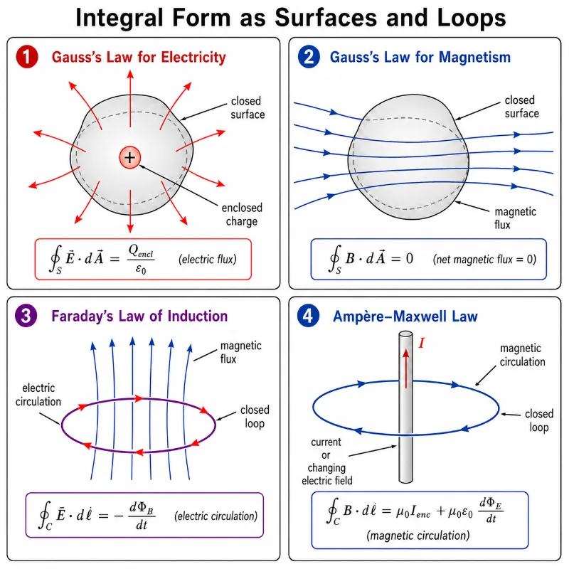
This illustration presents the integral form of Maxwell’s equations through four visual cases. The first panel shows electric flux through a closed surface enclosing charge. The second panel shows magnetic flux through a closed surface, with the net magnetic flux equal to zero. The third panel shows Faraday’s law, where changing magnetic flux is associated with electric circulation around a closed loop. The fourth panel shows the Ampère–Maxwell law, where current or a changing electric field is associated with magnetic circulation around a closed loop. The diagram helps students connect the mathematical integral forms with the physical ideas of surfaces, loops, flux, and circulation.
Why the Displacement Current Matters
Maxwell’s most important addition to Ampère’s law was the displacement current term. Before this addition, Ampère’s law described magnetic fields produced by electric currents. That was not enough for situations where electric fields change with time, such as between the plates of a charging capacitor.
In a capacitor circuit, conduction current flows in the wires, but no ordinary charge crosses the insulating gap between the plates. However, the electric field between the plates changes as the capacitor charges. Maxwell recognised that this changing electric field must also contribute to the magnetic field.
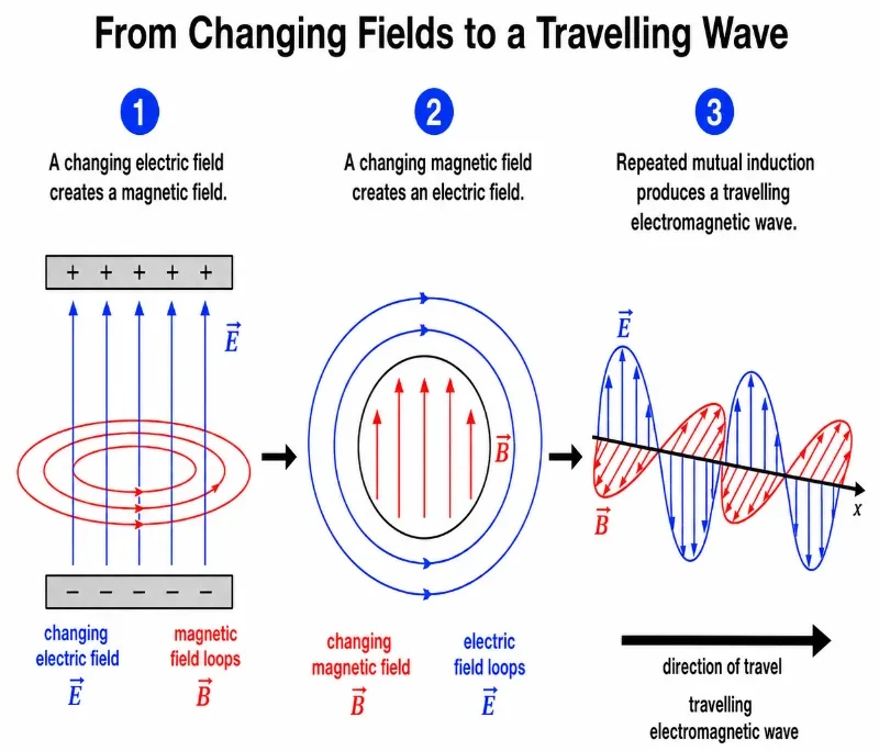
This insight made the theory consistent with charge conservation and allowed electromagnetic waves to exist in empty space. A changing electric field can produce a magnetic field, and a changing magnetic field can produce an electric field. Together, they can sustain a travelling wave.
Pictorial Illustration 3: Displacement Current in a Charging Capacitor
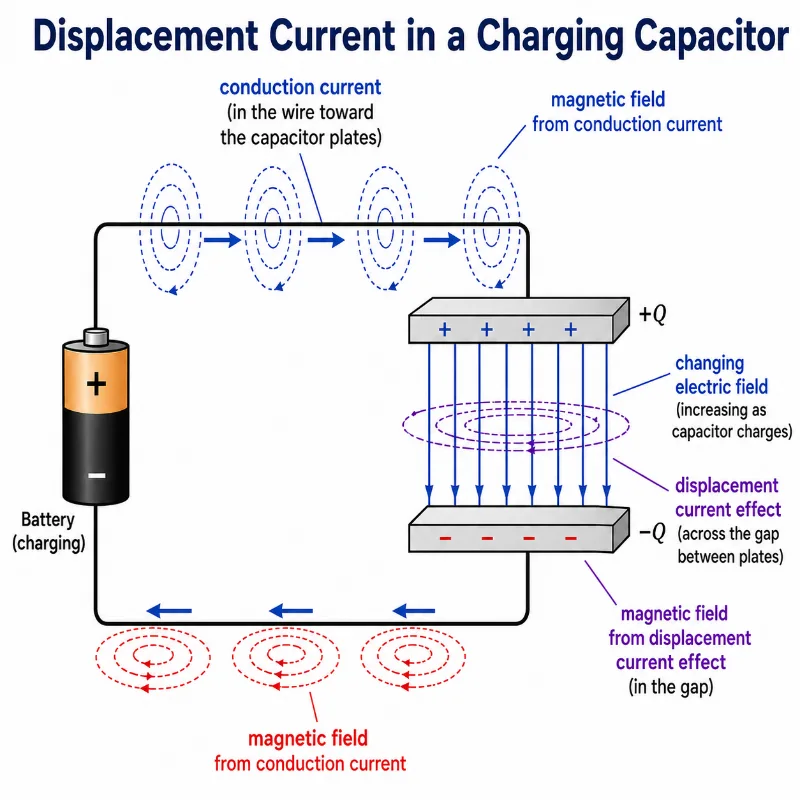
This illustration shows a capacitor being charged by a battery. Conventional conduction current flows through the wires toward and away from the capacitor plates, while the electric field between the plates changes as charge builds up. Although no ordinary conduction current crosses the gap between the plates, the changing electric field produces the displacement current effect, which acts as a source of magnetic field. The diagram helps students understand why Maxwell added the displacement current term to the Ampère–Maxwell law.
How Maxwell’s Equations Predict Electromagnetic Waves
In empty space, there is no charge density and no conduction current. This means \( \rho = 0 \) and \( \vec{J} = 0 \). Maxwell’s equations then show that changing electric and magnetic fields can generate one another.
From these equations, the electric and magnetic fields satisfy wave equations:
\( \nabla^2 \vec{E} = \mu_0\varepsilon_0\frac{\partial^2 \vec{E}}{\partial t^2} \)
\( \nabla^2 \vec{B} = \mu_0\varepsilon_0\frac{\partial^2 \vec{B}}{\partial t^2} \)
These equations have the form of wave equations, with wave speed:
\( c = \frac{1}{\sqrt{\mu_0\varepsilon_0}} \)
This speed matches the measured speed of light in vacuum. This was a profound result: light itself is an electromagnetic wave.
Pictorial Illustration 4: From Changing Fields to a Travelling Wave
Advanced Analytical Mechanics: Deriving the Electromagnetic Wave Equation
To mathematically prove Maxwell’s great insight that light is an electromagnetic wave, we must look at how the four equations interact in completely empty space. In a vacuum, where there are no net electric charges (\(\rho = 0\)) and no conduction currents (\(\mathbf{J} = 0\)), the differential equations decouple into a highly symmetrical form:
$$ \nabla \cdot \mathbf{E} = 0 \quad \text{and} \quad \nabla \cdot \mathbf{B} = 0 $$
$$ \nabla \times \mathbf{E} = -\frac{\partial \mathbf{B}}{\partial t} \quad \text{and} \quad \nabla \times \mathbf{B} = \mu_0\varepsilon_0\frac{\partial \mathbf{E}}{\partial t} $$To isolate the electric field vector field completely, we apply the vector calculus identity for the curl of a curl (\(\nabla \times (\nabla \times \mathbf{A}) = \nabla(\nabla \cdot \mathbf{A}) – \nabla^2\mathbf{A}\)) directly to Faraday’s Law:
$$ \nabla \times (\nabla \times \mathbf{E}) = \nabla \times \left( -\frac{\partial \mathbf{B}}{\partial t} \right) $$
$$ \nabla(\nabla \cdot \mathbf{E}) – \nabla^2\mathbf{E} = -\frac{\partial}{\partial t}(\nabla \times \mathbf{B}) $$By substituting the empty-space Gauss’s constraint (\(\nabla \cdot \mathbf{E} = 0\)) on the left side, and plugging the Ampère–Maxwell equation directly into the right side’s curl operator, the expression transforms into:
$$ 0 – \nabla^2\mathbf{E} = -\frac{\partial}{\partial t}\left( \mu_0\varepsilon_0\frac{\partial \mathbf{E}}{\partial t} \right) \Rightarrow \nabla^2\mathbf{E} = \mu_0\varepsilon_0\frac{\partial^2\mathbf{E}}{\partial t^2} $$This result is a classic three-dimensional second-order linear partial wave equation. Applying the identical sequence of vector curl operations to the Ampère–Maxwell law outputs a twin expression for the magnetic field component:
$$ \nabla^2\mathbf{B} = \mu_0\varepsilon_0\frac{\partial^2\mathbf{B}}{\partial t^2} $$In classical mechanics, any standard wave equation follows the structural format \(\nabla^2\psi = \frac{1}{v^2}\frac{\partial^2\psi}{\partial t^2}\), where \(v\) tracks the physical velocity of the propagating wavefront. Isolating this denominator parameter reveals that electromagnetic field perturbations ripple through empty space at a speed dictated entirely by the properties of the vacuum:
$$ v = \frac{1}{\sqrt{\mu_0\varepsilon_0}} \approx 3.00 \times 10^8 \text{ m/s} = c $$Theoretical Horizons: Magnetic Monopoles and Dual Gauge Symmetry
In classical electrodynamics, Gauss’s Law for Magnetism is rigidly locked at \(\nabla \cdot \mathbf{B} = 0\), representing the observational reality that cutting a bar magnet in half always yields a new paired North-South dipole, never an isolated pole. This structural asymmetry means that while electric fields can diverge outward from point charge entities, magnetic fields are trapped forming closed, circulating loops.
However, modern quantum field theory and grand unified models (GUTs) suggest that isolated magnetic point charges—known as magnetic monopoles—may have been created during the early stages of the universe. If a researcher were to securely detect a magnetic monopole with a localized magnetic charge density \(\rho_m\) and a corresponding magnetic current density \(\mathbf{J}_m\), Maxwell’s equations would transform into a state of perfect mathematical Dual Symmetry:
| Field Operation | Classical Form (No Monopoles) | Symmetric Dual Form (With Monopoles) |
|---|---|---|
| Electric Divergence | \(\nabla \cdot \mathbf{E} = \frac{\rho}{\varepsilon_0}\) | \(\nabla \cdot \mathbf{E} = \frac{\rho}{\varepsilon_0}\) |
| Magnetic Divergence | \(\nabla \cdot \mathbf{B} = 0\) | \(\nabla \cdot \mathbf{B} = \mu_0 \rho_m\) |
| Electric Curl | \(\nabla \times \mathbf{E} = -\frac{\partial \mathbf{B}}{\partial t}\) | \(\nabla \times \mathbf{E} = -\mu_0 \mathbf{J}_m – \frac{\partial \mathbf{B}}{\partial t}\) |
| Magnetic Curl | \(\nabla \times \mathbf{B} = \mu_0 \mathbf{J} + \mu_0 \varepsilon_0 \frac{\partial \mathbf{E}}{\partial t}\) | \(\nabla \times \mathbf{B} = \mu_0 \mathbf{J} + \mu_0 \varepsilon_0 \frac{\partial \mathbf{E}}{\partial t}\) |
Under this theoretical framework, rotating your calculation axes in the abstract charge space lets you map electric properties directly into magnetic parameters. Exploring this symmetry helps university-level students appreciate why theoretical physicists place immense value on structural beauty and mathematical elegance when drafting or modifying advanced cosmological laws.
Key Equations and What They Mean
\( \nabla \cdot \vec{E} = \frac{\rho}{\varepsilon_0} \)
Electric charge density is the source of electric field divergence.
\( \nabla \cdot \vec{B} = 0 \)
Magnetic field has no isolated source or sink in classical electromagnetism.
\( \nabla \times \vec{E} = -\frac{\partial \vec{B}}{\partial t} \)
A changing magnetic field produces a circulating electric field.
\( \nabla \times \vec{B} = \mu_0\vec{J} + \mu_0\varepsilon_0\frac{\partial \vec{E}}{\partial t} \)
Electric current and changing electric field produce a circulating magnetic field.
\( c = \frac{1}{\sqrt{\mu_0\varepsilon_0}} \)
The speed of electromagnetic waves in vacuum is determined by the electromagnetic constants of free space.
\( \vec{F} = q(\vec{E} + \vec{v} \times \vec{B}) \)
The Lorentz force law describes how electric and magnetic fields act on a charge moving with velocity \( \vec{v} \).
Maxwell’s Equations and the Lorentz Force
Maxwell’s equations describe how fields are produced and how they evolve. The Lorentz force law describes how those fields act on charges. Together, they form the practical engine of classical electromagnetism.
Maxwell’s equations answer questions such as: Where do electric and magnetic fields come from? How do they change? How do they travel? The Lorentz force law answers a different question: Once fields exist, what force do they exert on a charged particle?
This separation is powerful. It allows physicists and engineers to calculate fields first, then calculate how charges, currents, beams, plasmas, antennas, or materials respond to those fields.
Common Misconceptions about Maxwell’s Equations
Misconception 1: Maxwell’s Equations Are Only About Light
They do explain light as an electromagnetic wave, but they also describe electrostatics, magnetostatics, induction, circuits, antennas, waves, and electromagnetic energy flow.Misconception 2: The Equations Are Four Unrelated Rules
The four equations work together. Their full meaning appears when charges, currents, changing fields, and waves are treated as one system.Misconception 3: Magnetic Field Lines Start at North Poles
Magnetic field lines form closed loops. In classical electromagnetism, isolated magnetic monopoles are not part of Maxwell’s equations.Misconception 4: Displacement Current Is an Ordinary Current
Displacement current is not charge flowing through an insulator. It is the magnetic-field-producing effect of a changing electric field.Misconception 5: The Integral and Differential Forms Say Different Things
They express the same physics in different mathematical languages. One is local; the other describes behaviour over surfaces and loops.Misconception 6: Maxwell’s Equations Are Too Abstract to Be Practical
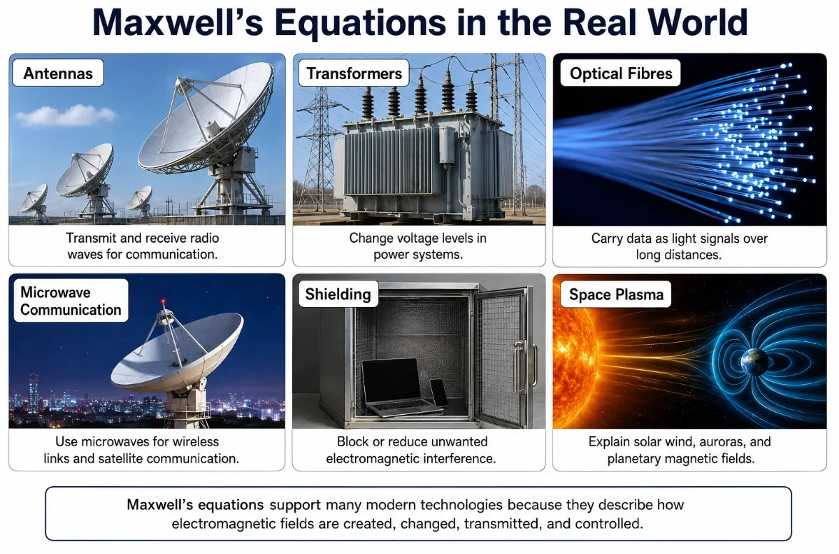
They are used in antennas, circuits, motors, transformers, optical fibres, lasers, microwave systems, satellites, and electromagnetic compatibility design.Practical Applications of Maxwell’s Equations
Maxwell’s equations are not only theoretical. They guide the design and understanding of many systems that move energy, signals, and information.
Antennas and Wireless Communication
Changing currents in antennas produce electromagnetic waves, and incoming waves drive currents in receiving antennas.Generators and Transformers
Faraday’s law explains induced electric fields, which are central to power generation and voltage transformation.Capacitors and High-Speed Circuits
The displacement current term helps explain magnetic fields and signal propagation in changing electric-field regions.Optics and Photonics
Light propagation, reflection, refraction, polarisation, waveguides, and optical fibres are all governed by electromagnetic field behaviour.Microwave and Radar Systems
Microwave cavities, waveguides, radar beams, and satellite communication depend on controlled electromagnetic waves.Medical and Scientific Imaging
X-ray imaging, MRI-related electromagnetic fields, optical imaging, and spectroscopy all rely on electromagnetic field principles.Electromagnetic Compatibility
Engineers use Maxwell’s equations to understand interference, shielding, grounding, and signal integrity in electronic systems.Plasma and Space Physics
Charged particles and electromagnetic fields interact strongly in plasmas, solar wind, auroras, and astrophysical environments.Real-World Illustration
Bridge to University Thinking
At school level, students often meet electricity and magnetism as separate topics: charges, currents, magnets, induction, and waves. At university level, Maxwell’s equations show that these ideas are parts of one field theory.
Students also begin to use vector calculus. Divergence measures how much a field spreads out from a point. Curl measures how much a field circulates around a point. Flux measures how much field passes through a surface. Circulation measures how much field runs around a path.
This mathematical language may feel demanding at first, but it is powerful because it allows one set of equations to describe fields in circuits, waves, materials, antennas, plasmas, and optical systems.
From Force to Field
Students move from calculating forces between charges to describing electric and magnetic fields throughout space.From Static to Dynamic
Static fields become time-varying fields, and time-varying fields can create new field patterns.From Circuits to Waves
The same electromagnetic laws help explain circuit behaviour, signal propagation, antennas, and electromagnetic radiation.From Classical to Modern Physics
Maxwell’s theory leads naturally to electromagnetic waves, special relativity, photons, and quantum electrodynamics.Quick Interactive Check
Quick Check: Reading Maxwell’s Equations
1. Which Maxwell equation says that electric charge is a source of electric field?
A. Gauss’s law for electricity
B. Gauss’s law for magnetism
C. Faraday’s law
D. Ampère–Maxwell law
Answer: A. Gauss’s law for electricity links electric field divergence to electric charge density.
2. Which Maxwell equation expresses the absence of isolated magnetic poles in classical electromagnetism?
A. Gauss’s law for electricity
B. Gauss’s law for magnetism
C. Faraday’s law
D. Lorentz force law
Answer: B. Gauss’s law for magnetism is written as \( \nabla \cdot \vec{B} = 0 \), meaning magnetic field has no isolated source or sink.
3. Which equation says that a changing magnetic field can produce a circulating electric field?
A. Faraday’s law
B. Gauss’s law for magnetism
C. Gauss’s law for electricity
D. Coulomb’s law
Answer: A. Faraday’s law states that a changing magnetic field produces a curling electric field.
4. Why was Maxwell’s displacement current term important?
A. It removed magnetic fields from the theory
B. It allowed only static charges to exist
C. It made changing electric fields a source of magnetic fields
D. It made electromagnetic waves impossible
Answer: C. Maxwell’s displacement current term shows that changing electric fields can produce magnetic fields, completing the symmetry needed for electromagnetic waves.
Review Questions and Answers
1. What are Maxwell’s equations?
Maxwell’s equations are four field equations that describe how electric and magnetic fields are produced by charges, currents, and changing fields.
2. What does Gauss’s law for electricity describe?
It describes how electric charge acts as a source or sink of electric field.
3. What does Gauss’s law for magnetism describe?
It states that the net magnetic flux through any closed surface is zero, meaning magnetic field lines do not begin or end at isolated magnetic charges.
4. What does Faraday’s law describe?
It describes how a changing magnetic field produces a circulating electric field.
5. What does the Ampère–Maxwell law describe?
It describes how electric current and changing electric field produce a circulating magnetic field.
6. What is displacement current?
Displacement current is the term associated with a changing electric field acting as a source of magnetic field.
7. Why do Maxwell’s equations predict electromagnetic waves?
They show that changing electric and magnetic fields can generate each other and propagate through space as waves.
8. What is the speed of electromagnetic waves in vacuum?
The speed is \( c = \frac{1}{\sqrt{\mu_0\varepsilon_0}} \), which equals the speed of light in vacuum.
9. What is the difference between differential and integral forms?
The differential form describes local field behaviour point by point, while the integral form describes field behaviour over surfaces and around loops.
10. How does the Lorentz force law relate to Maxwell’s equations?
Maxwell’s equations describe how fields are produced and evolve, while the Lorentz force law describes how those fields exert force on charged particles.
Thought-Provoking Questions and Answers
1. Why are Maxwell’s equations often described as a unification of electricity and magnetism?
They show that electric and magnetic fields are linked through sources, currents, and changing fields. Electricity and magnetism are therefore not separate subjects, but connected parts of electromagnetism.
2. Why was the prediction that light is an electromagnetic wave so important?
It connected optics with electromagnetism. Light was no longer only a visual phenomenon; it became part of a broader electromagnetic spectrum.
3. Why does the displacement current term make the theory more complete?
It allows changing electric fields to produce magnetic fields, which is essential for charge conservation and for electromagnetic waves to travel through vacuum.
4. Why is field language more powerful than force language alone?
Fields describe what exists throughout space and time, while forces describe the effect on a particular object. Field language makes it possible to study waves, energy flow, radiation, and distributed systems.
5. Why do Maxwell’s equations matter to engineering?
They help engineers design antennas, circuits, motors, transformers, waveguides, lasers, sensors, optical fibres, communication systems, and shielding strategies.
Numerical Problems and Solutions
Problem 1: An electric field passes through a closed surface with net enclosed charge \( Q_{\text{enc}} = 8.85 \times 10^{-9} \ \text{C} \). Find the electric flux through the surface.
Solution:
Using Gauss’s law:
\( \Phi_E = \frac{Q_{\text{enc}}}{\varepsilon_0} \)
\( \Phi_E = \frac{8.85 \times 10^{-9}}{8.85 \times 10^{-12}} \)
\( \Phi_E = 1.0 \times 10^3 \ \text{N m}^2/\text{C} \)
The electric flux is \( 1.0 \times 10^3 \ \text{N m}^2/\text{C} \).
Problem 2: The magnetic flux through a loop changes from \( 0.20 \ \text{Wb} \) to \( 0.05 \ \text{Wb} \) in \( 0.10 \ \text{s} \). Find the average induced emf magnitude.
Solution:
\( |\mathcal{E}| = \left| \frac{\Delta \Phi_B}{\Delta t} \right| \)
\( |\Delta \Phi_B| = |0.05 – 0.20| = 0.15 \ \text{Wb} \)
\( |\mathcal{E}| = \frac{0.15}{0.10} = 1.5 \ \text{V} \)
The average induced emf magnitude is \( 1.5 \ \text{V} \).
Problem 3: A long straight wire carries current \( I = 5.0 \ \text{A} \). Find \( \oint \vec{B} \cdot d\vec{l} \) around a loop enclosing the wire.
Solution:
Using Ampère’s law for steady current:
\( \oint \vec{B} \cdot d\vec{l} = \mu_0 I_{\text{enc}} \)
\( \oint \vec{B} \cdot d\vec{l} = (4\pi \times 10^{-7})(5.0) \)
\( \oint \vec{B} \cdot d\vec{l} \approx 6.3 \times 10^{-6} \ \text{T m} \)
The magnetic circulation is approximately \( 6.3 \times 10^{-6} \ \text{T m} \).
Problem 4: Using \( \mu_0 = 4\pi \times 10^{-7} \ \text{H/m} \) and \( \varepsilon_0 = 8.85 \times 10^{-12} \ \text{F/m} \), estimate \( c = \frac{1}{\sqrt{\mu_0\varepsilon_0}} \).
Solution:
\( c = \frac{1}{\sqrt{\mu_0\varepsilon_0}} \)
Substituting the constants gives approximately:
\( c \approx 3.0 \times 10^8 \ \text{m/s} \)
This is the speed of light in vacuum.
Problem 5: A charge \( q = 2.0 \times 10^{-6} \ \text{C} \) is placed in an electric field of magnitude \( E = 500 \ \text{N/C} \). If the charge is at rest, find the electric force on it.
Solution:
For a charge at rest, the magnetic part of the Lorentz force is zero.
\( F = qE \)
\( F = (2.0 \times 10^{-6})(500) \)
\( F = 1.0 \times 10^{-3} \ \text{N} \)
The force magnitude is \( 1.0 \times 10^{-3} \ \text{N} \).
Problem 6: A changing electric flux contributes a displacement current of \( 0.40 \ \text{A} \). What conduction current would produce the same magnetic circulation contribution in the Ampère–Maxwell law?
Solution:
The displacement current term contributes to magnetic circulation like an equivalent current.
Therefore, a conduction current of \( 0.40 \ \text{A} \) would produce the same current contribution.
The equivalent conduction current is \( 0.40 \ \text{A} \).
Summary
Maxwell’s equations are the four central field equations of classical electromagnetism. They describe how electric and magnetic fields are produced by charges, currents, and changing fields.
Gauss’s law for electricity links electric charge to electric field. Gauss’s law for magnetism states that magnetic field lines do not begin or end at isolated magnetic charges. Faraday’s law describes electric fields produced by changing magnetic fields. The Ampère–Maxwell law describes magnetic fields produced by currents and changing electric fields.
Maxwell’s displacement current term made the theory consistent and allowed electromagnetic waves to emerge naturally. From Maxwell’s equations, the predicted wave speed is \( c = \frac{1}{\sqrt{\mu_0\varepsilon_0}} \), the speed of light in vacuum.
For students, Maxwell’s equations are more than formulas. They are a compact map of how fields, sources, waves, energy, motion, and technology fit together.
Glossary
Maxwell’s equations: Four field equations describing how electric and magnetic fields are produced and how they change.
Electric field: A field that describes the electric force per unit positive charge.
Magnetic field: A field associated with moving charges, currents, magnets, and changing electric fields.
Divergence: A measure of how much a field spreads outward from or converges inward toward a point.
Curl: A measure of how much a field circulates around a point.
Flux: A measure of how much field passes through a surface.
Circulation: A measure of how much a field follows around a closed path.
Displacement current: The magnetic-field-producing effect of a changing electric field.
Electromagnetic wave: A travelling disturbance of electric and magnetic fields that can move through vacuum.
Lorentz force: The force on a charged particle due to electric and magnetic fields, given by \( \vec{F} = q(\vec{E} + \vec{v} \times \vec{B}) \).
Frequently Asked Questions
1. What are Maxwell’s equations in simple terms?
They are four laws that describe how electric and magnetic fields are created by charges, currents, and changing fields.
2. Why are Maxwell’s equations important?
They unify electricity, magnetism, induction, electromagnetic waves, light, and many technologies into one field theory.
3. Which equation did Maxwell complete?
Maxwell completed Ampère’s law by adding the displacement current term, which accounts for changing electric fields.
4. How do Maxwell’s equations predict light?
They imply wave equations for electric and magnetic fields in empty space, with wave speed equal to the speed of light.
5. What is the difference between electric and magnetic fields?
Electric fields act on charges, while magnetic fields act especially on moving charges and currents. In electrodynamics, the two fields are deeply connected.
6. Why are there no magnetic monopoles in Maxwell’s equations?
The equation \( \nabla \cdot \vec{B} = 0 \) says magnetic field lines do not start or end at isolated magnetic charges in classical electromagnetism.
7. Are Maxwell’s equations still used today?
Yes. They are essential in electrical engineering, communication systems, optics, photonics, antennas, circuits, and many areas of physics.
8. Are Maxwell’s equations replaced by quantum physics?
No. Quantum physics extends our understanding at microscopic scales, but Maxwell’s equations remain extremely accurate and useful in many classical and engineering situations.
Archived Version
An archived PDF version of this learning resource is available on Zenodo:
Maxwell’s Equations in Electrodynamics: An Open Educational Resource for University Preparation.