Advanced STEM OER

The Mathematics of 3D Printing Slicing

STL Geometry, Ray-Casting & Toolpath Slicing Foundations

Estimated Study Time: 75 Mins

Accreditation: WA1-WA5 | EUR-ACE

Author: Dr. Jacob Gan, PhD (Mich)

Core Competencies Learned

Calculate linear interpolation and intersection points for single triangular facets using vector equations.
Evaluate point inclusion using ray-casting algorithms and Even-Odd parity logic for complex geometric slices.
Understand the rasterization patterns and G-code coordinate generation required to translate continuous geometry into toolpaths.

To print a 3D digital object, software must first deconstruct it. Every additive manufacturing system works in layer-by-layer coordinates. Slicing translates a 3D boundary representation (B-Rep)—typically an STL (Stereolithography) mesh—into 2D paths a printhead or laser can trace. This module walks through the vector math, intersection proofs, and toolpath algorithms that govern this translation.

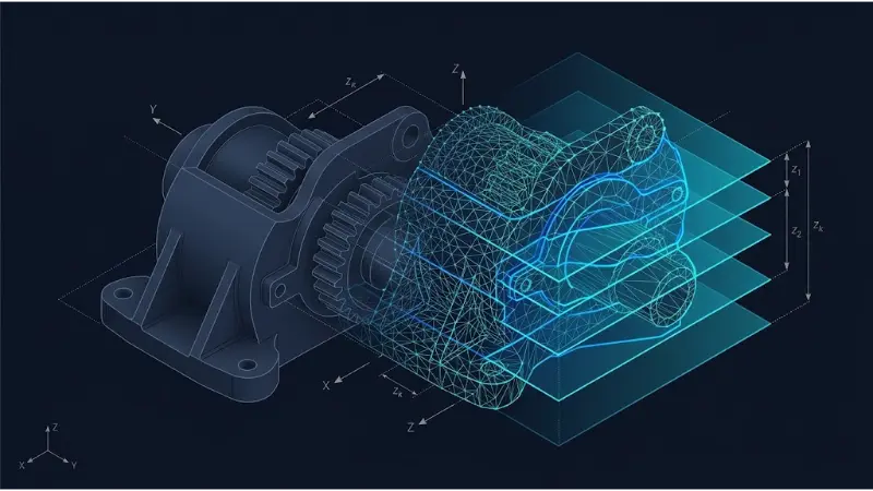
3D CAD mechanical model transitioning to a triangular STL wireframe mesh intersected by horizontal slicing planes

Figure 1: The slicing workflow. Solid CAD geometry is translated to a triangular STL wireframe, which is then intersected by parallel slicing planes at height $ z = z_k $.

Slicing Process Flow: Functional Architecture (IDEF0)

To analyze the slicing workflow as a systematic mathematical machine, we define its four functional boundaries:

Inputs (Left): STL 3D triangular mesh files containing facet vertices and surface normal vectors.

Controls (Top): Process parameters including slice thickness $\Delta z$, orientation, and infill geometry requirements.

Outputs (Right): Ordered, 2D slice boundary contours and raster infill coordinate sequences.

Mechanisms (Bottom): Slicing engines, linear interpolation math, and geometric parity algorithm solvers.

1. Slicing Mathematics and Edge Intersection

An STL file represents a 3D surface using an unorganized collection of triangular facets. Each facet $ i $ is defined by three vertices, $ V_1(x_1, y_1, z_1) $, $ V_2(x_2, y_2, z_2) $, and $ V_3(x_3, y_3, z_3) $, alongside an outward unit normal vector $ \mathbf{n} = (n_x, n_y, n_z) $.

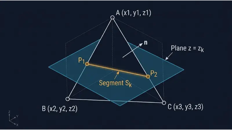
Individual triangular facet intersected by horizontal cutting plane z_k, showing vertices V1, V2, V3 and intersection points P1 and P2

Figure 2: Geometry of a facet-plane intersection. Slicing plane $ z = z_k $ intersects the triangle's edges at points $ P_1 $ and $ P_2 $.

When slicing at a horizontal plane $ z = z_k $, we first determine if a triangle intersects the plane. An intersection only exists if $ z_k $ is between the facet's minimum and maximum z-coordinates:

$$ \min(z_1, z_2, z_3) \leq z_k \leq \max(z_1, z_2, z_3) $$

To avoid degenerate edge cases (where the plane passes exactly through a vertex), we shift the plane by a tiny value $ \epsilon \approx 10^{-6}\text{ mm} $ if an exact match occurs.

For each intersected edge, we find the coordinate where the plane cuts it. Let an edge be defined by endpoints $ A(x_A, y_A, z_A) $ and $ B(x_B, y_B, z_B) $. We can represent any point $ P(x, y, z) $ on this edge using the parameter $ t \in [0, 1] $:

$$ P(t) = (1 - t)A + tB \quad \Rightarrow \quad z(t) = (1 - t)z_A + tz_B $$

To find the intersection at $ z(t) = z_k $, we solve for $ t $:

$$ z_k = z_A + t(z_B - z_A) \quad \Rightarrow \quad t = \frac{z_k - z_A}{z_B - z_A} $$

Because the intersection must lie between $ A $ and $ B $, $ t $ must fall in the interval $ (0, 1) $. Once we have $ t $, we calculate the 2D coordinates ($ x $, $ y $) of the intersection:

$$ x_k = x_A + t(x_B - x_A), \quad y_k = y_A + t(y_B - y_A) $$

Applying this calculation to the two intersected edges yields points $ P_1(x_{P1}, y_{P1}, z_k) $ and $ P_2(x_{P2}, y_{P2}, z_k) $. Together, these points form a 2D line segment $ S_k $ on the slicing plane. Collecting and connecting these segments for all intersected facets reconstructs the slice's 2D boundary.

Worked Example: Intersecting a Single Facet

Problem: Calculate the intersection of the triangle with vertices $ V_1(10, 10, 40) $, $ V_2(30, 10, 10) $, and $ V_3(20, 40, 20) $ and the slicing plane $ z_k = 25 $.

Step 1: Verify the intersection

The z-bounds are $ z_{min} = 10 $ and $ z_{max} = 40 $. Because $ z_k = 25 $ lies between 10 and 40, the facet intersects the plane.

Step 2: Find the intersected edges

Edge 1 ($ V_1 \to V_2 $): Span $ z_1 = 40 \to z_2 = 10 $. Contains $ z = 25 $.
Edge 2 ($ V_1 \to V_3 $): Span $ z_1 = 40 \to z_3 = 20 $. Contains $ z = 25 $.
Edge 3 ($ V_2 \to V_3 $): Span $ z_2 = 10 \to z_3 = 20 $. Does not reach $ z = 25 $.

Step 3: Calculate the intersection on Edge 1 ($ V_1 \to V_2 $)

$$ t_1 = \frac{z_k - z_1}{z_2 - z_1} = \frac{25 - 40}{10 - 40} = \frac{-15}{-30} = 0.5 $$ $$ x_{P1} = x_1 + t_1(x_2 - x_1) = 10 + 0.5(30 - 10) = 20 $$ $$ y_{P1} = y_1 + t_1(y_2 - y_1) = 10 + 0.5(10 - 10) = 10 $$ Point $ P_1 = (20, 10) $.

Step 4: Calculate the intersection on Edge 2 ($ V_1 \to V_3 $)

$$ t_2 = \frac{z_k - z_1}{z_3 - z_1} = \frac{25 - 40}{20 - 40} = \frac{-15}{-20} = 0.75 $$ $$ x_{P2} = x_1 + t_2(x_3 - x_1) = 10 + 0.75(20 - 10) = 17.5 $$ $$ y_{P2} = y_1 + t_2(y_3 - y_1) = 10 + 0.75(40 - 10) = 32.5 $$ Point $ P_2 = (17.5, 32.5) $.

Engineering Interpretation: These points define a boundary segment. The print nozzle must traverse the coordinate line from $ (20.0, 10.0) $ to $ (17.5, 32.5) $ at height $ z = 25 $.

2. Interior/Exterior Classification: The Ray-Casting Algorithm

To fill the intersected boundaries with solid patterns, the slicer must differentiate the interior from the exterior. It does this using the Ray-Casting Algorithm, which relies on the Even-Odd Parity Rule.

The algorithm shoots an imaginary horizontal ray from outside the print bed boundaries across the sliced cross-section. Slicers track every point where this ray intersects the boundary lines:

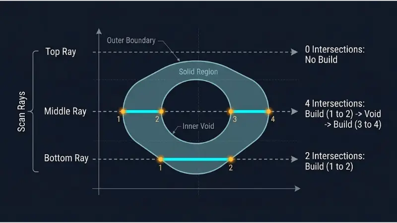
Ray-casting 2D horizontal test lines intersecting outer and inner boundaries of a slice

Figure 3: The Ray-Casting parity test. The middle ray has 4 intersections (crosses boundaries 1 and 2, exits back into space at 3, and terminates at 4).

For any point $ P_{test} $, we cast a horizontal ray $ R(t) = (x_{test} + t, y_{test}) $ for $ t \ge 0 $. We count how many times this ray intersects the polygon’s boundary edges. This count determines whether the point is inside the boundary:

Even count of intersections: The point is Outside the shape.
Odd count of intersections: The point is Inside the shape.

This simple logic allows the slicer to determine where to deposit material and where to avoid it (voids), ensuring proper boundary fills for any shape.

3. Rasterization & Toolpath Generation

Once the boundary is defined and the interior is identified, the slicer converts these areas into 2D motion paths. The toolpath is generally divided into two types: boundary perimeters and infill patterns.

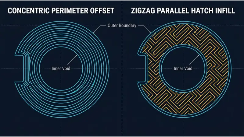
Side-by-side comparison of concentric perimeter offset vs zigzag parallel hatch infill on the same slice

Figure 4: Toolpath generation comparison. The perimeter-only offset strategy (left) contrasted with a perimeter and zigzag hatch infill pattern (right).

Boundary Perimeters: The printhead traces the outer shape, offsetting inward by half the nozzle's width ($ W / 2 $) to ensure accurate dimensions. This offset is computed by shifting the boundary vertices inward along their normal vectors.

Infill Rasterization: The solid areas inside the perimeters are filled using repeating geometric patterns. Slicers generate these paths by intersecting parallel line patterns with the boundary shapes, then trimming them to fit the interior using our ray-casting intersection math.

4. Interactive Slicing Mathematical Demonstration

Adjust the slicing parameters below to see how a horizontal plane ($z_k$) cuts through triangular facets and generates 2D segments in real time.

Active Computational Visualizer

V1(10, 10, 45) V2(50, 15, 10) V3(30, 40, 20)

Cutting Plane zk: 25 mm

Visualization Option:

Intersection Status: ACTIVE SEGMENT

P1: (18.6, 12.1) | P2: (19.0, 26.5)

5. Trade-Off Analysis: Slicing Slices vs Speed/Accuracy

Additive parameters involve continuous compromises. Adjusting slice height or geometry alters mechanical reliability, finish quality, and print time:

Slicing Setup Strategy	Primary Advantage	Key Technical Bottleneck	Optimization / Mitigation
Sub-0.1 mm Micro Slices	Excellent surface finish; reduced staircase effects on curves.	Extreme print times; increased risk of build failure due to cumulative errors.	Dynamic layer slicing; thinning layers only on curve sections.
Adaptive Dynamic Layering	Balances detail and speed by adjusting layer height based on local slope.	Complex toolpath transitions can lead to extrusion inconsistency.	Advanced firmware calibrations; adjusting material flow dynamically.
Concentric Outline Fills	High perimeter accuracy; minimizes tool vibration.	Poor interior filling; often creates internal gaps.	Hybrid infill; combining perimeters with internal zigzag paths.

6. Slicing Mathematics and Algorithms FAQ

Q1: What are the primary mathematical limitations of the STL file format for slicing?

STL files represent 3D surfaces as unorganized collections of flat triangles. They lack topological connectivity data (which vertices connect to which edges), forcing the slicer to reconstruct edge loops from scratch. This can lead to degenerate edges, tiny gaps, and geometric errors that require intensive computational repair before slicing can occur.

Q2: How does a slicer handle degenerate triangles or broken meshes?

If an STL has small gaps, overlapping facets, or non-manifold edges, the slicing plane may generate open, incomplete loops instead of closed boundaries. Slicers attempt to fix these by stitching nearby endpoints together within a tiny tolerance (e.g., 0.001 mm) or using volumetric pixel grid (voxel) techniques to reconstruction the geometry.

Q3: Why is the Jordan Even-Odd rule used instead of other point-in-polygon tests?

The Even-Odd rule is computationally efficient and robust, particularly for meshes with complex internal voids. It is easy to implement using 2D ray searches because it only requires counting intersections along a ray, rather than computing winding numbers, which require complex angular calculations.

Q4: How do numerical rounding errors affect the generated slice geometry?

Rounding errors can cause intersection points on shared facet edges to mismatch slightly, breaking the continuity of boundary loops. Standard slicers prevent this by using high-precision floats (64-bit doubles) and merging points that fall within a tiny spatial threshold.

Q5: How does adaptive slicing calculate changing layer heights?

Adaptive slicing analyzes the local slope of the mesh's surface normal vectors relative to the build axis (Z-axis). If it detects steep slope changes or fine vertical curves, it decreases the slice step size to minimize staircase effects; on straight vertical sections, it increases the step size to speed up the print.

Q6: Why are boundary perimeters usually printed before infill patterns?

Printing perimeters first establishes a precise external border, which improves dimensional accuracy and supports internal material flow. If infill is printed first, it can cause the perimeters to bulge slightly, reducing surface finish quality and part tolerances.

7. Slicing Mathematics Self-Assessment

Tier 1: Foundational Practice (True/False & Concept Multiple Choice)

Q1.1: If a horizontal slicing plane z_k passes through a triangular facet, can it intersect only one edge?

Answer: No. Under normal topological rules, a plane cutting through a closed triangular facet must intersect exactly two edges (producing an entry and exit point). An intersection at a single point is only possible if it touches exactly one vertex, which is a degenerate edge case generally resolved using a tiny epsilon shift.

Q1.2: A triangular facet has vertices with z-coordinates of 15.2, 10.4, and 30.1. Will it be intersected by slicing plane z_k = 15.0?

Answer: Yes. The Z-bounds of the facet are $ z_{min} = 10.4 $ and $ z_{max} = 30.1 $. Because the slicing plane $ z_k = 15.0 $ falls within this interval ($ 10.4 \leq 15.0 \leq 30.1 $), an intersection must exist.

Q1.3: Under the Even-Odd Parity rule, if a test ray has 5 intersections with a slice boundary, is the origin point inside or outside?

Answer: Inside. Since 5 is an odd number, the parity rule classifies the point as inside the boundary. Only even counts (like 0, 2, or 4) are outside the shape.

Q1.4: True or False: STL files contain explicit mathematical descriptions of curves like holes and cylinders.

Answer: False. STL files do not support true mathematical curves (like NURBS or analytical cylinders). All curved surfaces must be approximated (tessellated) using flat triangular facets, which introduces discretization errors.

Q1.5: The parameter 't' in linear interpolation equations must be in what interval for valid on-edge intersections?

Answer: The open interval $ (0, 1) $. A value of 0 or 1 indicates the intersection is exactly at one of the vertices, rather than on the edge segment itself. Slicers apply tiny coordinate shifts to avoid this and keep calculation robust.

Q1.6: Why does slicing a tilted, curved part produce a rough staircase pattern?

Answer: Slicing breaks the continuous, angled shape into discrete horizontal layers. The step-like staircase pattern is a natural artifact of building curved surfaces using vertical-sided layers of flat height.

Q1.7: When a test ray is exactly parallel to and touches a boundary edge, what issue does it create?

Answer: An intersection ambiguity. Ray-edge collinearity makes counting intersection points unreliable. Slicers solve this by slightly angling the ray or shifting its starting coordinate.

Q1.8: Why is checking minimum/maximum vertex z-height used as a preliminary filter before edge calculations?

Answer: Efficiency. Checking z-bounds allows the slicer to discard non-intersected facets immediately, avoiding the expensive linear calculations needed to verify edge cut details on the vast majority of triangles in a large mesh.

Tier 2: Applied Conceptual Cases & Slicer Debugging

Q2.1: Analyzing the geometric results of open-loop errors

Scenario: You inspect an G-code preview and find that some horizontal slices are filled only on one side, while other areas are completely un-filled or produce open tool paths.

Analysis: Unfilled sections suggest an unclosed (open) boundary loop. Slicers can only apply the even-odd test to complete, closed loops. If a gap exists, the scan ray fails to return the expected even/odd patterns, causing the software to misclassify filled areas. You can fix this by repairing the STL to stitch broken edges or using the slicer's self-repair options to bridge small gaps.

Q2.2: Managing vertices located exactly on slicing planes

Scenario: Slicing plane $ z_k = 20.0\text{ mm} $ aligns precisely with a flat shoulder of a part, causing slicing to fail or loops to misalign.

Analysis: Perfect alignment with vertices can result in ambiguous intersections (the plane touches a vertex, rather than cutting an edge), which disrupts the even-odd count. Slicers typically prevent this by applying a tiny shift to the cutting plane (e.g., $ z_k \pm 10^{-6}\text{ mm} $) to ensure the plane only intersects actual edges, resolving the geometric ambiguity.

Q2.3: Calculating tool orientation offsets for tight holes

Scenario: A sliced 10.0 mm hole in a printed model measures only 9.6 mm, but the outer dimensions of the part are perfectly accurate.

Analysis: Slicers shift toolpaths inward along surface normal vectors by the tool's radius ($ W / 2 $) to compensate for extrusion width. On small holes, material can over-squeeze inward due to rapid curvature, reducing the printed opening. You can compensate for this by applying shrinkage factors, adjusting extrusion flow, or modifying the CAD design to use slightly larger hole tolerances.

Q2.4: Speed-accuracy tradeoffs in curved surfaces

Scenario: A domed enclosure needs a smooth surface, but also requires a fast overall print time.

Analysis: Fixed 0.2 mm layers produce a fast print, but leave rough staircase patterns on the top dome curves. Using 0.05 mm layers solves the staircase effect, but dramatically increases print times. An adaptive slicer solves this by varying the layer height—using thin layers on the dome's slopes to preserve detail, and thick layers on the vertical walls to keep print times fast.

Q2.5: The computational cost of mesh density

Scenario: A high-poly organic mesh takes several minutes to slice, causing the slicing software to freeze.

Analysis: Large STL files contain millions of triangles, many with dimensions smaller than the print nozzle's diameter. Intersecting, sorting, and linking this level of geometry strains memory and processor time. Simplify the mesh in CAD or reduce its triangle count prior to slicing to decrease the calculation burden without affecting the final print quality.

Q2.6: Choosing infill strategy based on tool travel time

Scenario: Compare toolhead acceleration and travel times between concentric perimeters and zigzag infill on a large square layer.

Analysis: Concentric perimeters produce smooth, continuous paths that minimize decelerations, making them highly efficient for boundary printing. However, filling a large internal area concentrically can leave poor material connections at the center. Zigzag infill is easier to pattern and ensures consistent density, but requires the toolhead to stop and reverse direction frequently, which can increase travel times on large prints.

Q2.7: Overhang failures on un-supported slopes

Scenario: An unsupported 60° overhanging slope sags and creates loose, unbonded threads on the underside of the print.

Analysis: Slicing overhanging geometry causes each layer to shift outward, leaving part of the new extrusion unsupported in thin air. At angles past a critical limit (usually 45°), the lack of support causes gravity to pull the molten material downward before it can bond. Activating support structures or modifying the design to keep overhangs under 45° prevents these drooping failures.

Tier 3: Slicing Mathematics & Numerical Exercises

Q3.1: Finding linear intersection on an angled edge

Problem: Given an edge $ V_1(0, 0, 10) \to V_2(20, 10, 40) $, find the (x, y) intersection coordinates at slicing height $ z_k = 25 $.

Steps: 1. Calculate interpolation parameter $ t $: $$ t = \frac{z_k - z_1}{z_2 - z_1} = \frac{25 - 10}{40 - 10} = \frac{15}{30} = 0.5 $$ 2. Substitute $ t $ into coordinate equations: $$ x = x_1 + t(x_2 - x_1) = 0 + 0.5(20 - 0) = 10 $$ $$ y = y_1 + t(y_2 - y_1) = 0 + 0.5(10 - 0) = 5 $$

Engineering Interpretation: The intersection is $ (10.0, 5.0) $. This precise coordinate represents one of the endpoint bounds on the slice layer.

Q3.2: Calculating the interpolation ratio t for custom planes

Problem: An edge is defined by $ P_1(5, 5, 12.5) \to P_2(15, 25, 22.5) $. Find $ t $ for intersection planes $ z_k = 15.0 $, $ z_k = 17.5 $, and $ z_k = 20.0 $.

Steps: Calculate for each height using the formula $ t = \frac{z_k - z_1}{z_2 - z_1} $, where $ z_2 - z_1 = 22.5 - 12.5 = 10.0 $: * For $z_k = 15.0$: $$t = \frac{15.0 - 12.5}{10.0} = 0.25$$ * For $z_k = 17.5$: $$t = \frac{17.5 - 12.5}{10.0} = 0.50$$ * For $z_k = 20.0$: $$t = \frac{20.0 - 12.5}{10.0} = 0.75$$

Engineering Interpretation: Slicing this edge at equal height intervals results in equal stepping of interpolation parameters, demonstrating consistent toolpath advancement.

Q3.3: Resolving degenerate coordinate vertex intersection

Problem: Slicing plane $z_k = 25.0$ passes through a facet with vertices $V_1(10, 10, 25.0)$, $V_2(20, 20, 15.0)$, and $V_3(10, 30, 20.0)$.

Steps: 1. Slicing plane aligns exactly with $V_1$ ($z = 25.0$), creating a potential edgecase mismatch. 2. Set $\epsilon = 10^{-6}$ to adjust $z_k$ slightly below 25.0 to resolve the ambiguity: $$z_k' = z_k - \epsilon = 24.999999 \text{ mm}$$ The adjusted plane falls below 25.0, removing V1 as a plane intersection point and ensuring normal calculation on the two vertical edges without triggering degenerate software loops.

Engineering Interpretation: This adjustment resolves potential open-loop errors, preventing the software from crashing on V1 and ensuring the slicer continues without gaps.

Q3.4: Finding coordinates on an angled edge

Problem: Determine the coordinates of $P_{mid}$ where the slicing plane $z_k = 18.0$ intersects edge $V_1(5, 8, 12.0) \to V_2(15, 20, 22.0)$.

Steps: 1. Solve for interpolation parameter $t$: $$t = \frac{18.0 - 12.0}{22.0 - 12.0} = \frac{6.0}{10.0} = 0.6$$ 2. Substitute $t = 0.6$ into coordinates equations: $$x_{mid} = 5 + 0.6(15 - 5) = 5 + 6 = 11.0$$ $$y_{mid} = 8 + 0.6(20 - 8) = 8 + 7.2 = 15.2$$ The intersection coordinate is $(11.0, 15.2, 18.0)$.

Engineering Interpretation: Accurate calculation at $(11.0, 15.2)$ prevents micro-stepping and ensures exact coordinate matching along the toolpath.

Q3.5: Estimating G-code segments for outer outlines

Problem: Generate the segment output G-code starting at intersection point $P_1(15.0, 20.0)$ and ending at $P_2(35.0, 40.0)$ on slice $z = 15.0$. Set speed $F = 1800$ and estimate a volumetric extrusion value $E = 1.45$.

Steps: Draft the ordered travel parameters based on standard machine G-code format: 1. Position the printhead without extruding (G0) to the starting intersection point:

G0 X15.0 Y20.0 Z15.0 F1800.0

2. Trace and extrude (G1) to the end intersection point:

G1 X35.0 Y40.0 E1.45

Engineering Interpretation: The G-code translates intersection geometry into coordinate path commands, feeding vector logic directly to the machine's motors.

Q3.6: Estimating staircase errors on angled profiles

Problem: Compute the stair step width $\delta_x$ for a 60° slope angle (relative to horizontal) with layer heights $h_1 = 0.2\text{ mm}$ and $h_2 = 0.05\text{ mm}$.

Steps: 1. Relationship for step width is defined by slope angle $\theta$: $$\tan(\theta) = \frac{h}{\delta_x} \quad \implies \quad \delta_x = \frac{h}{\tan(\theta)}$$ 2. For $h_1 = 0.2\text{ mm}$: $$\delta_x = \frac{0.2}{\tan(60^\circ)} = \frac{0.2}{1.732} = 0.1155\text{ mm}$$ 3. For $h_2 = 0.05\text{ mm}$: $$\delta_x = \frac{0.05}{\tan(60^\circ)} = \frac{0.05}{1.732} = 0.0289\text{ mm}$$

Engineering Interpretation: Reducing the layer height from 0.2 mm to 0.05 mm shrinks the stair step width by 75%, significantly improving surface finish on sloped surfaces.

Interactive Education Hub Navigation

Expand your knowledge by browsing other advanced resources in the Additive Manufacturing track:

MODULE 01 (You are Here)

Slicing Mathematics & Toolpaths

The definitive guide on translating unorganized 3D STL meshes into layer-by-layer motion paths and parity classifications.

MODULE 02

Overhang Limit & Support Physics

Learn how shear limits and thermal transfer requirements dictate the placement and math of support structures.

MODULE 03

The ISO/ASTM 52900 7 Categories

Analyze process characteristics and hardware mechanisms across all seven official ASTM AM process types.

The Mathematics of 3D Printing Slicing: STL Geometry, Ray-Casting & Toolpaths