
After decades of teaching students in different disciplines, one lesson becomes clear: many academic difficulties arise not from the subject itself, but from weak mathematical foundations. Students often struggle in physics, engineering, economics, computing, and even parts of the social sciences not because the ideas are beyond them, but because the mathematical relationships underlying those ideas are unfamiliar or poorly understood.
Mathematics is more than a collection of formulas. It is a way of thinking about relationships, patterns, change, and uncertainty. Once students grasp a few fundamental mathematical ideas, they begin to see the same structures appearing across many university subjects. These recurring ideas form part of the intellectual toolkit used in modern science, engineering, economics, and data analysis.
The ten ideas presented below are not advanced techniques. Instead, they are core mathematical concepts that repeatedly appear in university study. Understanding them early helps students move beyond memorizing formulas and begin to think more confidently and analytically about the problems they encounter in higher education.
These ideas appear repeatedly across science, engineering, economics, and data analysis. Together they form a foundation for mathematical thinking at the university level.
Foundations Hub
Navigate the central mathematical gateway designed to bridge secondary school mathematics with university rigor.
Calculus Primer
Master limits, differentiation, and integration to model dynamic systems, velocities, and area accumulations.
Linear Algebra Primer
Discover vectors, matrices, and linear transformations that underpin data science and multi-dimensional geometry.
Probability & Statistics
Learn how to measure uncertainty, evaluate conditional events, and build predictive statistical models.
Concept 1. Mathematics as a Language of Relationships
At its heart, mathematics is a language for describing relationships between quantities. Rather than studying numbers in isolation, mathematics focuses on how one quantity depends on another. This perspective allows patterns to be expressed clearly and analyzed systematically.
For example, the distance travelled by a moving object may depend on time, the total cost of purchasing items may depend on the number of items bought, and a student’s final course grade may depend on scores from assignments, tests, and examinations. In each case, the central task is to understand how changes in one variable influence another.
Consider a simple example involving ticket purchases. Suppose the total cost of a purchase depends on the number of tickets bought, the cost of each ticket, and a fixed processing fee.
= 7 × $12.50 + $9 = $96.50
This simple example illustrates how mathematics expresses relationships between quantities. When the number of tickets changes, the total cost changes as well. By representing the relationship using symbols and equations, mathematics allows us to calculate outcomes clearly and predict how a result will change when one of the inputs is modified.
We can also express this relationship symbolically. Let C represent the total cost, n the number of tickets, t the ticket price, and f the processing fee. The relationship can then be written as
This compact symbolic expression captures the same relationship in a general form. By representing relationships using symbols, equations, tables, and graphs, mathematics provides a concise way to describe complex systems. This ability to express relationships precisely allows mathematics to serve as a foundation for subjects ranging from physics and engineering to economics, computing, and the social sciences.
Question 1
Suppose the total cost of purchasing tickets is described by the equation C = nt + f, where C is the total cost, n is the number of tickets purchased, t is the price per ticket, and f is a fixed service charge. Which statement best describes the relationship represented by this equation?
Question 2
A farmer observes that increasing the amount of fertilizer applied to crops tends to increase the crop yield. Which statement best describes this situation?
Concept 2. Functions: Describing How One Quantity Depends on Another
A central idea in mathematics is the concept of a function. A function describes how one quantity depends on another. When the value of one variable changes, the value of another variable responds according to a defined relationship.
In mathematical language, a function assigns an output value to each allowed input value. The input is often called the independent variable, while the resulting quantity is called the dependent variable. This simple idea allows many real-world relationships to be expressed clearly and analyzed systematically.
In its simplest form, a function may describe how a single variable determines another. For example, the distance travelled by a moving object may depend on time, or the total cost of purchasing items may depend on the number of items bought. Such relationships are often written in the form:
This notation means that the value of y is determined by the value of x according to a rule represented by the function f.
However, most real systems involve more than one influencing factor. In many scientific, engineering, and economic situations, the outcome depends on several variables interacting together. A more realistic representation may therefore involve multiple inputs affecting a single result:
Many of these relationships can be expressed using equations, which provide explicit rules connecting the variables.
A simple example from algebra is a quadratic function that describes how one quantity depends on another:
In this equation, x is the input variable and y is the resulting output. Changing the value of x changes the value of y according to the rule defined by the function.
In physics, the distance travelled by an object moving with constant acceleration can be described by the equation
Here, s represents distance travelled, u is the initial velocity, a is acceleration, and t is time. The distance therefore depends on several variables simultaneously.
In economics, a simple demand relationship may be expressed as
In this equation, Q represents the quantity demanded and P represents price. The equation shows that demand decreases as price increases.
These examples illustrate how functions and equations describe relationships between variables in many disciplines. Learning to interpret such relationships is one of the key mathematical skills needed for university study.
Question 3
A function assigns exactly one output value to each input value. Which of the following situations best represents a function?
Question 4
Suppose a function describes how the temperature of a cup of tea changes over time. What does the function allow us to determine?
Concept 3. Linear Relationships: The Simplest Mathematical Model
One of the most important mathematical ideas encountered across university subjects is the linear relationship. A linear relationship describes a situation in which one quantity changes at a constant rate with respect to another.
The most familiar form of a linear relationship is written as
where
y = the dependent variable
x = the independent variable
m = the slope (constant rate of change)
c = the intercept (value of y when x = 0)

This diagram illustrates a typical linear relationship on Cartesian axes. The straight line rises at a constant rate, indicating that the dependent variable changes proportionally with the independent variable. The point where the line intersects the vertical axis represents the intercept, which is the value of the dependent variable when the independent variable is zero. Linear models such as this are widely used in mathematics, physics, engineering, and economics to represent relationships where one quantity changes at a constant rate with respect to another.
A simple real-world example appears in the ticket purchase scenario introduced earlier. Suppose the total cost of buying tickets depends on the number of tickets purchased, the cost of each ticket, and a fixed processing fee. This relationship can be written as
If each ticket costs $12.50 and the processing fee is $9, the relationship becomes

Linear graph of C = 12.5n + 9 illustrating how total cost increases with the number of tickets purchased while including a fixed processing fee.
This diagram shows the linear relationship C = 12.5n + 9 plotted on a coordinate plane. The horizontal axis represents the number of tickets purchased n, and the vertical axis represents the total cost C. The straight line rises at a constant rate, indicating that each additional ticket increases the total cost by a fixed amount. The line intersects the vertical axis at 9, representing the fixed processing fee charged even when no tickets are purchased. This graph visually demonstrates how linear equations can model real-world relationships where a constant rate of change and a starting value are both present.
Here, n represents the number of tickets purchased and C represents the total cost. This equation is linear: each additional ticket increases the total cost by the same fixed amount ($12.50), while the processing fee ($9) remains constant. In this case, the ticket price plays the role of the slope and the processing fee acts as the intercept.
Linear relationships appear widely in many fields of study. For example, in physics, the distance travelled by an object moving at constant velocity is described by
where s is distance, v is velocity, and t is time. The distance increases proportionally with time.
In economics, revenue can also be modeled linearly when price per unit remains constant:
where R is revenue, p is price per unit, and Q is the quantity sold. If the price remains fixed, revenue increases proportionally with the number of units sold.
Linear models are powerful because they are simple, easy to analyze, and often provide a good first approximation of real systems. Many scientific and economic models begin by assuming linear behaviour before introducing more complex nonlinear effects.
Understanding linear relationships helps students recognize patterns, interpret graphs, and build mathematical models — essential skills across science, engineering, economics, and data analysis.
Question 5
A linear relationship between two variables produces what type of graph?
Question 6
If the cost of printing posters is given by C = 5x, what does the number 5 represent?
Concept 4. Nonlinear Relationships: When Change Is Not Constant
While linear relationships describe situations where quantities change at a constant rate, many real-world systems behave in more complex ways. In these situations, the rate of change itself varies as the variables change. Relationships of this type are called nonlinear relationships.
A simple example of a nonlinear relationship is the quadratic function
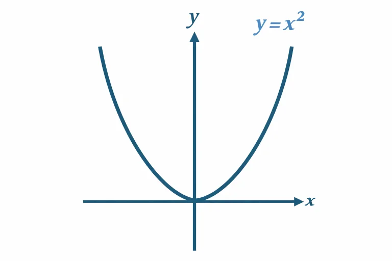
In this equation, x is the input variable and y is the resulting output. As the value of x increases, the value of y increases more rapidly because the output depends on the square of x. The graph of this relationship forms a curved shape rather than a straight line, showing that the rate of change is not constant.
Nonlinear relationships appear frequently in science and engineering. For example, the distance travelled by an object moving under constant acceleration is described by
Here s represents distance, u is the initial velocity, a is acceleration, and t is time. Because of the squared term t2, the distance does not increase linearly with time. Instead, the rate at which distance increases becomes larger as time progresses.

This diagram illustrates the nonlinear relationship between distance and time for an object moving with constant acceleration. The horizontal axis represents time t, while the vertical axis represents distance s. The curve follows the equation s = ut + ½at2 and passes through the origin, showing that when time begins at zero the displacement is zero. Unlike a straight line, the curve bends upward, indicating that distance increases more rapidly as time progresses due to acceleration. This visual representation helps students recognize how quadratic terms produce curved graphs and why motion under constant acceleration cannot be described by a simple linear model.
Nonlinear behaviour also appears in many natural and social systems. For example, population growth or compound interest often follows an exponential pattern:
In this equation, P(t) represents the population at time t, P0 is the initial population, r is the growth rate, and e is a mathematical constant approximately equal to 2.718. Exponential growth differs from quadratic growth because the rate of increase becomes proportional to the current value of the quantity itself.

This graph illustrates an exponential relationship between the quantity P and time t. The curve represents the equation:
The value of P grows increasingly rapidly as time increases. Unlike linear relationships, where change occurs at a constant rate, exponential growth accelerates because the rate of increase is proportional to the current value of the quantity.
The vertical axis represents P, while the horizontal axis represents t. Such exponential patterns appear in many real-world contexts, including population growth, continuous compound interest, the spread of information, and certain biological processes.
Recognizing nonlinear relationships is important because many real systems do not behave in simple proportional ways. Understanding these patterns prepares students for further study in calculus, physics, engineering, economics, and many other fields. Because nonlinear relationships can be difficult to understand from equations alone, graphical representation becomes an important tool for visualizing how quantities change.
Question 7
Which of the following situations is most likely to produce a nonlinear relationship?
Question 8
If the graph of a relationship is curved rather than straight, what does this usually indicate?
Concept 5: Multi-Variable Thinking
In school mathematics, many problems involve only one variable. For example, a function such as y = x2 describes how a single quantity changes with another. However, most real-world systems depend on several variables interacting at the same time.
Understanding how multiple variables influence an outcome is one of the most important mathematical skills needed for university studies.
When More Than One Factor Matters
In many situations, a result depends on several inputs. For example:
- In physics, the distance travelled depends on speed and time.
- In economics, profit depends on price, demand, and cost.
- In engineering, structural stress depends on force, material properties, and geometry.
- In environmental science, temperature may depend on latitude, altitude, and time of year.
Instead of a function like:
we now consider functions such as:
or even:
This means the output depends on several variables simultaneously.
Visualizing Multi-Variable Relationships
A function with two variables can often be visualized as a surface. For example, the function:
forms a curved surface called a paraboloid. Each point on the surface corresponds to a pair of input values (x, y) and the resulting output z.

In this surface, the value of z increases as either x or y moves away from zero. The result is a smooth bowl-shaped surface that rises in all directions from the origin. Such surfaces frequently appear in multivariable calculus, physics, optimization, and engineering when studying systems influenced by two independent variables.
Not all surfaces curve in the same direction. Some relationships rise in one direction while falling in another. For example:

This surface curves upward along the x-direction and downward along the y-direction, creating a characteristic saddle shape. At the origin the surface forms neither a maximum nor a minimum; instead it forms a saddle point where curvature changes direction. Such surfaces appear frequently in multivariable calculus, optimization, geometry, and many physical systems where quantities depend on multiple variables.
Surfaces like these help visualize how several variables interact to determine an outcome.
Why This Idea Matters
University-level problems rarely depend on just one variable. Engineers, scientists, and economists constantly analyze systems where multiple factors interact. For example:
- Designing an aircraft wing involves airflow speed, pressure, angle, and geometry.
- Climate models involve temperature, humidity, ocean currents, and atmospheric circulation.
- Machine learning models may depend on hundreds or thousands of variables.
Learning to think in terms of multiple variables allows us to understand complex systems and build predictive models.
Key Insight
Many real-world problems are not controlled by a single factor. Mathematics allows us to describe how several variables work together to determine an outcome.
The ability to analyse relationships involving multiple variables is therefore a crucial step toward advanced study in science, engineering, economics, and data science.
To analyze such systems mathematically, we often represent quantities as vectors that describe both magnitude and direction.
Question 9
Suppose the fuel consumption of a car depends on both speed and road slope. What type of relationship does this represent?
Question 10
Weather conditions depend on temperature, pressure, humidity, and wind. What does this illustrate about many real-world systems?
Concept 6: Vectors
In many areas of mathematics and science, quantities are not described by magnitude alone. Some quantities also have a direction. These quantities are called vectors.
Understanding vectors is essential for university studies in physics, engineering, computer graphics, robotics, and data science.
Scalars and Vectors
A scalar is a quantity that has magnitude only. Examples include:
- Mass
- Temperature
- Energy
- Time
A vector, in contrast, has both magnitude and direction. Examples include:
- Velocity
- Force
- Displacement
- Acceleration
For example, saying a car travels at 60 km/h describes only its speed. Saying it travels at 60 km/h toward the north describes a vector quantity because both magnitude and direction are specified.
Representing Vectors
Vectors are often represented as arrows. The length of the arrow represents the magnitude, while the direction of the arrow indicates the direction of the quantity.
Mathematically, a vector in two dimensions can be written as:
where:
vx represents the horizontal component
vy represents the vertical component
In three-dimensional space, a vector may be written as:
These components describe how far the vector extends in each spatial direction.
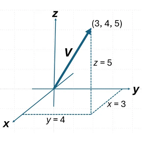
This diagram illustrates a three-dimensional vector v = (3, 4, 5) originating from the coordinate origin in a Cartesian coordinate system. The vector extends to the point (3, 4, 5), indicating movement of 3 units in the x-direction, 4 units in the y-direction, and 5 units in the z-direction. Dashed projection lines show how the point relates to each coordinate axis, helping visualize the vector’s components along the x, y, and z directions.
Such representations are fundamental in linear algebra, physics, and engineering, where vectors are used to describe quantities that have both magnitude and direction, such as displacement, velocity, and force.
Vector Addition
Vectors can be combined by adding their components. If:
then:
Graphically, vector addition can be visualized using the tip-to-tail method, where one vector begins at the endpoint of another.

This diagram illustrates the geometric interpretation of vector addition. Vector U originates at the origin, while vector V begins at the tip of U, demonstrating the tip-to-tail method of addition. The resultant vector U + V connects the origin directly to the final endpoint of the two vectors combined.
This visual method is widely used in physics and engineering to understand how forces, velocities, and displacements combine to produce a resultant effect.
Why Vectors Matter
Vectors are fundamental tools for describing physical systems and geometric relationships. They are used in:
- Physics to represent forces, motion, and fields
- Engineering to analyze structures and fluid flows
- Computer graphics to describe positions and movements
- Machine learning to represent high-dimensional data
- Robotics to model motion and orientation
Many advanced mathematical ideas—including matrices, linear algebra, and optimization—build directly on vector concepts.
Key Insight
Vectors allow mathematics to describe quantities that involve both magnitude and direction. This simple idea opens the door to powerful tools used across science, engineering, computing, and modern data analysis.
Once quantities are represented using vectors and mathematical relationships, the next step is understanding how these quantities change. This leads naturally to the concept of rates of change.
Question 11
Which quantity requires both magnitude and direction to be fully described?
Question 12
Two forces act on an object in different directions. Why are vectors needed to combine them?
Concept 7: Rates of Change
Many real-world processes involve quantities that change over time or with respect to another variable. Understanding how quickly a quantity changes is one of the central ideas in mathematics and science. This idea is known as the rate of change.
Rates of change appear in many contexts. In physics, velocity describes how quickly position changes with time. In economics, marginal cost measures how production cost changes as output increases. In biology, population growth describes how the size of a population changes over time.
Average Rate of Change
The simplest way to measure change is to compare two values. Suppose a quantity changes from f(x1) to f(x2). The average rate of change between these two points is:
This expression measures how much the function value changes for each unit change in the variable. In graphical terms, it represents the slope of the straight line connecting the two points on the graph.
Instantaneous Rate of Change
In many situations, we want to know the rate of change at a specific point rather than across a large interval. For example, the speed of a car at a particular moment is more informative than its average speed over an hour.
Mathematics captures this idea using the concept of the derivative. The derivative measures the instantaneous rate of change of a function.
For a function f(x), the derivative is written as f'(x) and represents the slope of the tangent line to the curve at that point.

This diagram shows the graph of the quadratic function y = x2 together with several tangent lines drawn at different points along the curve. Each tangent line represents the instantaneous rate of change of the function at that specific value of x.
Near the vertex at x = 0, the tangent line is horizontal because the slope is zero. As we move farther away from the origin, the tangent lines become steeper because the rate of change increases. This visual interpretation helps explain how derivatives measure how rapidly a function changes at a particular point.
A Simple Example
Consider the function f(x) = x2. The derivative of this function is:
This means the rate at which the function changes depends on the value of x. As x becomes larger, the function increases more rapidly.
Rates of Change in Multivariable Functions
Many real-world systems depend on more than one variable. In such cases the function may be written as f(x, y). For example, consider the function:
This function depends on two independent variables. The rate of change therefore depends on the direction in which we move on the surface defined by the function. Since there are infinitely many possible directions, the function can have infinitely many possible rates of change at a single point.
To study this situation systematically, mathematics introduces the idea of partial derivatives. A partial derivative measures how the function changes with respect to one variable while the other variables are held constant.
The partial derivative with respect to x is written as:
This tells us how the function changes when x varies while y remains fixed.
Similarly, the partial derivative with respect to y is:
This measures how the function changes when y varies while x is kept constant. Partial derivatives therefore allow us to analyse complex systems where several variables interact simultaneously.
Why Rates of Change Matter
Rates of change are fundamental to many scientific and technical disciplines.
- Physics uses derivatives to describe motion and acceleration.
- Engineering uses rates of change to analyze heat transfer, fluid flow, and electrical signals.
- Economics uses marginal analysis to study production and pricing decisions.
- Biology uses growth rates to model populations and chemical reactions.
These ideas form the foundation of calculus, which is one of the most important mathematical tools used in university-level study.
Key Insight
Rates of change allow us to measure how quantities evolve. By understanding how a system changes at each moment, mathematics provides powerful tools for predicting future behavior and designing complex systems.
If derivatives describe how quantities change at each moment, another mathematical idea explains how these changes accumulate over time. This leads to the concept of accumulation and integration.
Question 13
If the position of a moving object changes over time, what does the rate of change of position represent?
Question 14
On a graph of distance versus time, what does the slope of the graph represent?
Concept 8: Accumulation
While rates of change describe how quantities evolve, another important mathematical idea focuses on how quantities build up over time. This idea is known as accumulation.
Many real-world problems involve quantities that gradually accumulate. For example, rainfall accumulates in a reservoir, small financial transactions accumulate into total savings, and continuous energy consumption accumulates into total electricity usage.
Adding Many Small Contributions
Accumulation often occurs through the addition of many small contributions. If a quantity changes continuously, we can approximate the total accumulation by adding many small pieces together.
For example, suppose a car’s speed varies over time. The total distance travelled can be estimated by adding together many small distances covered during short time intervals.
In mathematics, this idea leads to the concept of summing small pieces:
As the pieces become smaller and more numerous, the approximation becomes increasingly accurate.

This diagram shows a smooth increasing function plotted on Cartesian axes with several equal-width rectangles beneath the curve. The height of each rectangle is determined by the function value at the right edge of the interval, so the top right corner of every rectangle touches the curve. The sum of the areas of these rectangles approximates the total area under the curve, illustrating the fundamental idea of accumulation that leads to integration in calculus.
Area Under a Curve
One common way to visualize accumulation is through the area under a graph. If a function describes a rate—such as speed, growth rate, or energy flow—the total accumulated quantity can often be represented as the area under the curve of that function. For example:
- If a graph shows velocity versus time, the area under the curve represents total distance travelled.
- If a graph shows power versus time, the area represents total energy used.
- If a graph shows growth rate versus time, the area represents total growth.
This geometric interpretation makes accumulation easier to understand and apply.

This illustration shows a smooth increasing function f(x) plotted on Cartesian axes. The shaded region extends from x = 0 to x = b and lies beneath the curve. This shaded area represents the definite integral:
which measures the accumulated quantity of the function over the interval from 0 to b.
Such accumulated areas appear in many contexts, including distance from velocity, energy from power, and total growth from a rate of change.
From Accumulation to Integration
The mathematical tool used to compute accumulation precisely is called the integral. In calculus, integration provides a systematic way to combine infinitely many tiny contributions into a single total quantity.
Integration is widely used in:
- Physics to calculate work, energy, and mass distributions
- Engineering to analyze systems that evolve continuously
- Economics to compute total production or cumulative costs
- Statistics to determine probabilities from continuous distributions
Key Insight
If rates of change tell us how quantities evolve, accumulation tells us how those changes build up over time. Together, these two ideas—rates of change and accumulation—form the foundation of calculus and many powerful mathematical tools used in science and engineering.
Question 15
If velocity is plotted against time, what does the area under the curve represent?
Question 16
Why do mathematicians divide areas into many small pieces when calculating accumulation?
Concept 9: Probability
Not all phenomena in the world can be predicted with certainty. Weather systems, financial markets, biological processes, and even the outcomes of games involve elements of uncertainty. Mathematics provides tools to study and quantify this uncertainty through the concept of probability.
Probability allows us to measure how likely an event is to occur. Instead of predicting a single outcome with certainty, we evaluate the likelihood of different possible outcomes.
Understanding Probability
Probability is usually expressed as a number between 0 and 1.
- A probability of 0 means the event cannot occur.
- A probability of 1 means the event is certain to occur.
- A probability between 0 and 1 represents varying degrees of likelihood.
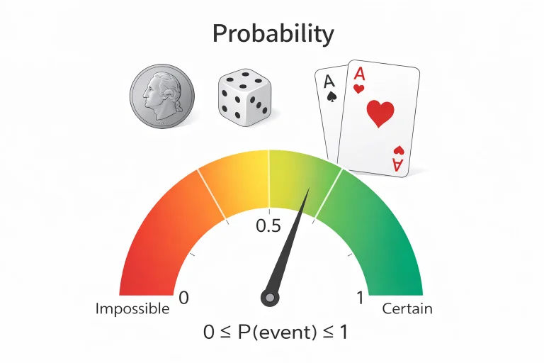
This illustration introduces the concept of probability as a numerical measure of uncertainty. A probability scale runs from 0, representing an impossible event, to 1, representing a certain event. Everyday random experiments such as tossing a coin, rolling a die, and drawing cards are shown to illustrate situations where outcomes cannot be predicted with certainty. Probability values between 0 and 1 describe varying degrees of likelihood and form the foundation for reasoning about uncertainty in science, engineering, finance, and data analysis.
For example, when tossing a fair coin, there are two equally likely outcomes: heads or tails. The probability of obtaining heads is:
This means that, over many repeated trials, heads is expected to occur about half of the time.
Random Experiments
A random experiment is an action whose outcome cannot be predicted with certainty in advance. Examples include:
- Tossing a coin
- Rolling a die
- Drawing a card from a shuffled deck
- Observing whether a machine component fails within a given time
Although the exact outcome of a single experiment is uncertain, probability theory allows us to understand the long-term behavior of repeated experiments.
Two Coin Toss Outcomes
When a fair coin is tossed twice, there are four possible outcomes. Each outcome represents a sequence of heads (H) and tails (T).
| First Toss / Second Toss | Heads | Tails |
|---|---|---|
| Heads | HH | HT |
| Tails | TH | TT |
Each outcome occurs with probability ¼ for a fair coin.
This table represents the sample space for two successive coin tosses. The rows correspond to the outcome of the first toss and the columns correspond to the outcome of the second toss. The four possible sequences—HH, HT, TH, and TT—are displayed in the table. Because the coin is fair, each outcome has equal probability.
Conditional Probability
Sometimes the probability of an event changes when we know that another event has already occurred. This idea is called conditional probability. It describes the probability of one event given that another related event has already happened.
The conditional probability of event A given that event B has occurred is written as P(A | B). Mathematically, conditional probability is defined as:
This formula means that we focus only on the situations where event B occurs, and then determine how often event A also occurs within those situations.

Conditional probability is widely used in fields such as statistics, medicine, finance, and artificial intelligence, where new information continuously updates the likelihood of future events.
For example, suppose we draw one card from a standard deck of 52 cards.
- Event A: The card is a King.
- Event B: The card is a Face Card.
There are 12 face cards in the deck (J, Q, K of four suits), and 4 of them are Kings. If we already know the card is a face card, the probability that it is a King becomes:
Probability in Real-World Applications
Probability plays a crucial role in many fields.
- Statistics uses probability to analyze data and draw conclusions.
- Finance uses probability to estimate investment risks.
- Engineering uses probability to study system reliability.
- Medicine uses probability to interpret diagnostic tests and clinical outcomes.
- Artificial intelligence uses probability to make predictions from data.
Because many real-world systems involve uncertainty, probability provides a mathematical framework for making informed decisions.
Key Insight
Probability allows mathematics to describe uncertainty in a systematic way. By measuring likelihood and analyzing repeated events, probability helps us understand patterns within randomness and make rational decisions in uncertain situations.
Question 17
When tossing a fair coin, what is the probability of obtaining heads?
Question 18
Why is probability useful in scientific and engineering studies?
Concept 10: Optimization
In many real-world situations, we want to find the best possible outcome among many alternatives. This process of finding the most efficient, most profitable, or least costly solution is known as optimization.
Optimization is one of the most powerful applications of mathematics. It allows us to determine how to allocate resources, design systems efficiently, and make informed decisions.
Finding Maximum and Minimum Values
Optimization problems often involve identifying the maximum or minimum value of a quantity. For example:
- An engineer may want to design a beam that is as strong as possible while using the least amount of material.
- A company may want to maximize profit while minimizing production costs.
- A logistics planner may want to determine the shortest delivery route between multiple locations.
- A scientist may want to find the conditions that produce the highest reaction yield.
In each case, mathematics helps identify the best solution under given constraints.
Optimization in Mathematics
Many optimization problems are expressed using functions. The goal is to determine the value of a variable that produces the highest or lowest value of the function.
For example, if a quantity is described by a function f(x), we may wish to find the value of x that makes f(x) as large or as small as possible. In calculus, derivatives are often used to identify these optimal points.
Constraints in Optimization
In real-world problems, we rarely have complete freedom when searching for the best solution. Most decisions must satisfy certain limitations or requirements. These limitations are known as constraints.
Constraints restrict the range of values that the variables in a problem can take. Instead of searching for the best solution everywhere, we search only among solutions that satisfy the required conditions. For example:
- A company may want to maximize profit, but production cannot exceed available raw materials.
- An engineer may want to design the strongest structure possible, but the total weight must remain below a safety limit.
- A delivery company may want to minimize travel distance, but vehicles must follow existing roads.
Mathematically, an optimization problem often involves finding the maximum or minimum value of a function while satisfying one or more constraints:
Constraints may be expressed as equations or inequalities that the variables must satisfy. The set of all values that satisfy the constraints is called the feasible region. The optimal solution must lie within this region.

This diagram illustrates the idea of optimization under constraints. The curve represents a function whose value changes with x. However, instead of searching for the maximum or minimum over all possible values of x, the solution is restricted to the interval between x = a and x = b shown as the shaded region. In constrained optimization, the optimal value must be found within this feasible region defined by the constraints.
Applications Across Disciplines
Optimization appears throughout science, engineering, and business.
- Engineering design uses optimization to improve efficiency and safety.
- Economics uses optimization to study consumer behavior and production decisions.
- Machine learning uses optimization algorithms to train predictive models.
- Operations research uses optimization to schedule production and transportation.
- Architecture and urban planning use optimization to balance cost, functionality, and sustainability.
These methods allow complex problems to be approached systematically.
Key Insight
Optimization transforms mathematics from a tool for describing systems into a tool for improving them. By analyzing relationships between variables and constraints, mathematics helps identify the most effective solutions to practical problems.
Optimization is one of the many ways mathematics helps transform understanding into action. The broader connections between these ideas become clearer when we view them together as part of the larger structure of university mathematics.
Question 19
What is the goal of optimization in mathematics?
Question 20
Why do many optimization problems include constraints?
How These 10 Ideas Connect in University Mathematics

This concept map summarizes how the ten mathematical ideas discussed on this page relate to one another. Mathematical thinking begins with relationships and functions, which lead to linear and nonlinear models. These ideas extend to multi-variable systems and vectors, which describe complex systems and directional quantities. Calculus concepts such as rates of change and accumulation build on these foundations, while probability and optimization provide tools for dealing with uncertainty and making effective decisions in real-world applications.
The ten concepts presented on this page are not isolated topics. Together, they form a connected framework that underlies much of the mathematics used in university studies across science, engineering, economics, computing, and many other disciplines.
Each idea builds naturally on the previous ones. As students progress through these concepts, they begin to see how mathematical thinking evolves from simple relationships into powerful tools for analyzing complex systems and making informed decisions.
From Simple Relationships to Mathematical Models
Mathematical thinking often begins by identifying relationships between quantities. Functions provide a systematic way to express these relationships. Linear and nonlinear models allow us to describe how one variable influences another, revealing patterns that can be analyzed, visualized, and predicted.
In many real-world situations, however, systems depend on several interacting variables rather than a single quantity. Multi-variable thinking extends these ideas and allows complex phenomena—such as climate systems, financial markets, or engineering designs—to be represented mathematically.
Describing Direction and Motion
Vectors introduce the ability to represent quantities that have both magnitude and direction. This concept is essential in fields such as physics, engineering, robotics, and computer graphics, where direction and movement are fundamental.
Vector ideas also form the foundation for more advanced mathematical tools such as matrices, coordinate transformations, and linear algebra, which are widely used in modern scientific computing and data analysis.
Understanding Change and Accumulation
Rates of change and accumulation form the conceptual core of calculus. Rates of change allow us to measure how quantities evolve from one moment to the next, while accumulation allows us to determine how many small changes combine into a total effect over time.
Together, these ideas provide powerful tools for analyzing motion, growth, energy transfer, fluid flow, and many other dynamic processes encountered in science and engineering.
Dealing with Uncertainty and Decision Making
Probability introduces another dimension of mathematical thinking. Instead of focusing only on deterministic relationships, probability allows us to analyze situations involving randomness and uncertainty.
Optimization then uses mathematical tools to identify the best possible outcome among many alternatives. Whether maximizing efficiency, minimizing cost, or improving performance, optimization helps translate mathematical understanding into practical decision-making.
Seeing the Big Picture
As students progress into university-level mathematics, these ideas begin to connect more deeply. Linear algebra builds on vectors and multi-variable systems. Calculus extends rates of change and accumulation. Statistics grows from probability. Optimization combines many of these concepts to solve complex real-world problems.
Together, these ten ideas form a conceptual map of the mathematical tools that support modern science, engineering, economics, and data-driven disciplines. Students who become comfortable with these foundational ideas will find the transition to university mathematics far smoother and more meaningful.
Interactive Math Concept Explorer & Optimizer
Use the interactive simulator below to manipulate linear models, nonlinear quadratic growth, and constrained optimization bounds. Observe how slope, curvature, and feasibility regions interact in real time.
Interactive Model & Feasible Region Visualizer
Interactive Review Questions
Test your understanding of the foundational concepts using the toggle questions below.
Why are linear models considered the starting point for scientific modeling?
What distinguishes a scalar quantity from a vector quantity?
How does conditional probability restrict the sample space of an experiment?
Frequently Asked Questions
Why do many university students struggle with introductory STEM courses?
Difficulties usually arise not from the core domain concepts, but from unfamiliarity with how mathematical relationships (such as rates of change, vectors, or multivariable dependencies) describe those concepts.
What is partial differentiation in multi-variable calculus?
Partial differentiation measures how a multi-variable function changes with respect to one single variable while holding all other input variables strictly constant.
How does constrained optimization differ from unconstrained optimization?
Unconstrained optimization searches across all domain values for peaks or valleys, whereas constrained optimization restricts the search to a specific "feasible region" defined by physical or financial limits.
Comprehensive Practice Module
Section 1: Foundational Review Questions
- In the ticket pricing equation C = nt + f, what does the variable f represent?Answer: It represents the fixed processing fee or service charge (the vertical y-intercept).
- Define a mathematical function in terms of inputs and outputs.Answer: A function is a rule that assigns exactly one output value to each valid input value.
- What type of geometric graph is produced by a linear equation of the form y = mx + c?Answer: A straight line with constant slope m.
- Give an example of a scalar quantity and a vector quantity from physics.Answer: Speed is a scalar quantity (magnitude only); velocity is a vector quantity (magnitude and direction).
- What does the derivative f'(x) measure on a function graph?Answer: The instantaneous rate of change or slope of the tangent line at point x.
- How is continuous accumulation calculated geometrically from a rate curve?Answer: By computing the area under the curve using definite integration.
- What range of numerical values can probability take?Answer: Real numbers between 0 (impossible event) and 1 (certain event) inclusive.
- What is a "feasible region" in constrained optimization?Answer: The set of all possible points that satisfy all problem constraints simultaneously.
Section 2: Analytical & Scenario-Based Questions
- Suppose a crop yield increases as fertilizer is added, but adding too much fertilizer causes toxicity and reduces yield. What type of model best captures this?Answer: A nonlinear (quadratic or parabolic) model with a single peak maximum point.
- A boat moves East at 4 knots while a river current pushes North at 3 knots. Why cannot the combined velocity be calculated by simple scalar addition (4 + 3 = 7)?Answer: Velocity is a vector quantity. Perpendicular components must be added vectorially using the Pythagorean theorem, yielding a resultant speed of 5 knots.
- Why is a partial derivative used instead of a standard derivative when evaluating heat distribution across a metal plate?Answer: Temperature varies across multiple spatial coordinates (x, y). Partial derivatives measure the temperature gradient along one axis while holding the other fixed.
- If a factory's marginal revenue equals marginal cost at a certain output level, what does calculus reveal about total profit?Answer: The profit derivative is zero (dP/dq = 0), indicating a potential critical point for profit optimization (maximum profit).
- How does knowing that a drawn card is a Face Card alter the conditional probability that it is a King?Answer: It shrinks the sample space from 52 cards down to 12 face cards, raising the probability from 4/52 (1/13) to 4/12 (1/3).
- Why do linear models often serve as good approximations in engineering despite real systems being nonlinear?Answer: Over very small operating ranges, smooth nonlinear curves appear approximately linear (tangent line approximation).
- If a car's velocity graph is a horizontal line at 60 km/h for 2 hours, how does the definite integral calculate total distance?Answer: The integral computes the area of a rectangle of height 60 and width 2, yielding 120 km.
Section 3: Numerical Problems with Step-by-Step Solutions
- A printing company charges a flat setup fee of $15 plus $0.20 per printed booklet. Write the linear equation for total cost C and find the cost for 250 booklets.Solution:
Linear model: C = 0.20n + 15
Substitute n = 250:
C = (0.20 × 250) + 15 = 50 + 15 = 65
Total Cost = $65.00 - An object's displacement is given by s(t) = 2t2 + 3t + 5. Find its instantaneous velocity at t = 4 seconds.Solution:
Velocity v(t) = ds/dt = 4t + 3
Substitute t = 4:
v(4) = (4 × 4) + 3 = 16 + 3 = 19
Velocity = 19 units/s - Calculate the magnitude of the 2D vector u = (6, 8).Solution:
Magnitude |u| = √(ux2 + uy2)
|u| = √(62 + 82) = √(36 + 64) = √100 = 10
Magnitude = 10 units - Find the resultant vector w = a + b where a = (3, -2, 5) and b = (1, 7, -2).Solution:
Add corresponding components:
wx = 3 + 1 = 4
wy = -2 + 7 = 5
wz = 5 + (-2) = 3
Resultant Vector w = (4, 5, 3) - Given the multi-variable function f(x, y) = 4x2y + 3y3, find the partial derivative with respect to x (∂f / ∂x).Solution:
Treat y as a constant:
(∂ / ∂x)(4x2y) = 8xy
(∂ / ∂x)(3y3) = 0
∂f / ∂x = 8xy - Evaluate the total accumulated area under the rate curve f(x) = 3x2 from x = 0 to x = 3.Solution:
Definite integral ∫03 3x2 dx
Antiderivative F(x) = x3
Evaluate at limits: F(3) - F(0) = 33 - 03 = 27 - 0
Accumulated Area = 27 units2 - A pair of fair 6-sided dice are rolled. What is the probability that the sum of the numbers is equal to 7?Solution:
Total outcomes = 6 × 6 = 36
Outcomes summing to 7: (1,6), (2,5), (3,4), (4,3), (5,2), (6,1) = 6 outcomes
Probability = 6 / 36 = 1 / 6
Probability = 1/6 (approx. 0.167) - Find the value of x that maximizes the profit function P(x) = -2x2 + 12x - 5.Solution:
Take derivative and set to zero: P'(x) = -4x + 12 = 0
-4x = -12 → x = 3
Second derivative test: P''(x) = -4 (concave down, maximum confirmed)
Optimal input x = 3 units