
Digital image processing forms the mathematical and algorithmic bedrock of computer vision. Long before high-level deep neural networks interpret visual scenes, raw optical signals captured by sensors must be digitized, conditioned, filtered, enhanced, compressed, and segmented into structured spatial information.
Whether analyzing biometric fingerprint ridge structures, performing non-destructive X-ray inspection in manufacturing, detecting defects on printed circuit boards (PCBs), or identifying pupil-iris boundaries in biometric security scanners, classical 2D digital image processing algorithms provide deterministic, interpretable, and computationally efficient foundations for extracting pictorial patterns.
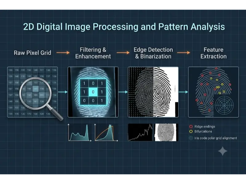
Unlike 3D scene reconstruction or temporal video tracking, 2D image analysis operates directly on planar discrete intensity arrays. By applying spatial domain convolution, frequency-domain Fourier transforms, contrast histogram equalization, mathematical morphology, and geometric moment invariants, engineers transform noisy digital bitmaps into quantitative structural descriptors.
Image Representation and Quantization
A continuous physical image captured by an optical camera or X-ray detector is converted into a digital representation through two fundamental operations: spatial sampling and amplitude quantization.
Spatial sampling discretizes the continuous 2D spatial coordinates (x, y) into an M × N grid of discrete spatial picture elements called pixels. Amplitude quantization maps continuous light intensity or radiation flux at each pixel coordinate into discrete numeric intensity levels bounded by a fixed bit depth b.
For a grayscale image with a bit depth of b bits per pixel, the available discrete intensity levels L are:
$$
L = 2^b
$$For a standard 8-bit grayscale image, L = 256 intensity levels ranging from 0 (pure black) to 255 (pure white).
Color Spaces and Multi-Channel Representation
Color images store intensity measurements across multiple spectral bands. The most common color models include:
- RGB (Red, Green, Blue): Primary additive color space used in hardware displays and raw camera sensors, representing images as three 2D spatial matrices IR(x, y), IG(x, y), and IB(x, y).
- HSV / HSI (Hue, Saturation, Value/Intensity): Decouples color chromaticity (Hue and Saturation) from luminance intensity (Value). This separation is advantageous for illumination-invariant feature tracking and segmentation.
- Grayscale Luminance Conversion: Standard ITU-R BT.601 perceptual weighting converts RGB triples to a single luminance channel Y based on human eye spectral sensitivity:
Principles of Image Compression and File Storage
Raw uncompressed digital images consume significant memory bandwidth and storage space. An uncompressed RGB image with spatial resolution W × H at 8 bits per channel requires a raw memory footprint calculated as:
$$
\text{Memory Size (Bytes)} = W \times H \times 3
$$For a 4K resolution frame (3840 × 2160 pixels), uncompressed storage equals 24.88 Megabytes (MB). To optimize transmission and storage, image compression algorithms convert raw pixel maps into compressed file formats.
Lossless Compression (.png, .tiff)
Lossless compression preserves 100% of original pixel data, guaranteeing exact bit-for-bit reconstruction upon decompression.
- PNG (Portable Network Graphics): Employs 2D spatial prediction filtering followed by the DEFLATE compression algorithm (a combination of LZ77 dictionary encoding and Huffman entropy coding). It is ideal for sharp line art, document OCR, and biometric prints where degradation is unacceptable.
- TIFF (Tagged Image File Format): Flexible raster container supporting uncompressed, LZW (Lempel-Ziv-Welch), or lossless Huffman encoding, widely used in professional archive photography, high-resolution X-ray diagnostics, and satellite orthophotos.
Lossy Compression (.jpg, .webp)
Lossy compression achieves dramatic file size reductions (e.g., 10:1 to 20:1 compression ratios) by discarding visually redundant high-frequency details that human visual perception rarely detects.
The standard JPEG (.jpg) pipeline executes five sequential mathematical stages:
- Color Space Transformation: Converts RGB into YCbCr (Luminance Y, Blue-Difference Cb, Red-Difference Cr).
- Chrominance Subsampling: Downsamples Cb and Cr channels (e.g., 4:2:0 scheme) because human vision is less sensitive to spatial color variations than luminance.
- Discrete Cosine Transform (DCT): Divides each channel matrix into non-overlapping 8×8 pixel blocks and applies 2D DCT, converting spatial pixel intensities into 64 spatial frequency coefficients.
- Quantization: Divides DCT coefficients by a lossy quantization matrix and rounds to integers. High-frequency spatial coefficients are truncated to zero, driving compression.
- Entropy Encoding: Encodes zero-quantized coefficients using Zig-Zag scanning, Run-Length Encoding (RLE), and Huffman coding.
WebP (.webp): A modern format offering both lossy and lossless modes. Lossy WebP utilizes intra-frame spatial predictive coding (derived from the VP8 video codec) to outperform JPEG by 25%–34% in compression efficiency at equivalent visual quality.
Interactive Quick Review: Sampling, Quantization & File Formats
Test your understanding of digital image representations, bit depths, and compression mechanics before exploring spatial domain contrast operations:
Quick Review Verification
1. What is the fundamental difference between PNG and JPEG compression algorithms?
Answer: PNG uses lossless compression combining spatial prediction with DEFLATE (LZ77 + Huffman) to preserve exact pixel data, whereas JPEG uses lossy compression involving Discrete Cosine Transforms (DCT) and coefficient quantization to achieve smaller file sizes by discarding high-frequency detail.
2. How many distinct intensity levels can be represented in an 8-bit single-channel grayscale image?
Answer: L = 28 = 256 distinct intensity levels (integer values ranging from 0 to 255).
Spatial Domain Processing & Contrast Enhancement
Spatial domain image processing operates directly on image pixel values f(x, y) to produce a modified output image g(x, y):
$$
g(x,y) = T[f(x,y)]
$$where T is a spatial transformation operator defined over a single pixel or a local spatial neighborhood.
Point Operations and Contrast Stretching
Point operations apply intensity transformations independently to each pixel based solely on its current gray level. Linear contrast stretching scales poor dynamic range inputs to span the full available range [0, L – 1]:
$$
g(x,y) = \frac{f(x,y) – f_{\min}}{f_{\max} – f_{\min}} \times (L – 1)
$$Histogram Equalization and CLAHE
The normalized image histogram represents the discrete probability density function (PDF) pr(rk) of gray levels in an image:
$$
p_r(r_k) = \frac{n_k}{MN}
$$where nk is the number of pixels with gray level rk, and MN is total image pixel count.
Global Histogram Equalization (HE) applies a cumulative distribution function (CDF) transformation mapping sk = T(rk) to distribute pixel intensities uniformly, maximizing overall global image entropy and contrast:
$$
s_k = (L – 1) \sum_{j=0}^{k} p_r(r_j) = \frac{L – 1}{MN} \sum_{j=0}^{k} n_j
$$CLAHE (Contrast Limited Adaptive Histogram Equalization): Global HE often over-amplifies noise in homogenous areas (such as X-ray tissue backgrounds). CLAHE addresses this by dividing images into small local contextual blocks (e.g., 8×8 tiles), computing local histograms, and clipping histogram counts above a predefined contrast clip limit before redistributing pixels. Neighboring tiles are merged using bilinear interpolation to eliminate boundary artifacts.
Spatial Filtering and Linear Convolution
Spatial domain filtering modifies a pixel’s intensity based on values in its surrounding spatial neighborhood using a small 2D coefficient matrix known as a filter kernel or mask w of size m × n.
2D spatial convolution of image f with kernel w is expressed as:
$$
g(x,y) = f(x,y) * w(x,y) = \sum_{s=-a}^{a} \sum_{t=-b}^{b} w(s,t) f(x-s, y-t)
$$where a = (m – 1)/2 and b = (n – 1)/2.
- Box Filter (Mean Blur): Replaces central pixel with the arithmetic average of neighborhood pixels, smoothing noise but blurring sharp edges.
- Gaussian Smoothing Filter: Weighs neighboring pixels using a 2D Gaussian spatial probability distribution, providing isotropic noise suppression while preserving structural gradients better than a box filter:
- Median Filtering (Non-Linear Order-Statistic Filter): Replaces the center pixel with the statistical median value within the local window. It is uniquely effective at eliminating impulse noise (salt-and-pepper noise) while preserving sharp object boundary edges intact.
Frequency Domain Analysis & Image Transforms
Frequency domain analysis decomposes 2D spatial images into constituent sinusoidal spatial frequencies. Rapid intensity variations (edges, fine lines, noise) correspond to high spatial frequencies, while smooth, slowly varying background regions correspond to low spatial frequencies.
2D Discrete Fourier Transform (2D DFT)
The 2D DFT transforms an M × N spatial domain image f(x, y) into its frequency spectrum representation F(u, v):
$$
F(u,v) = \sum_{x=0}^{M-1} \sum_{y=0}^{N-1} f(x,y) e^{-j 2\pi \left(\frac{ux}{M} + \frac{vy}{N}\right)}
$$The Inverse 2D DFT reconstructs spatial domain pixels from frequency coefficients:
$$
f(x,y) = \frac{1}{MN} \sum_{u=0}^{M-1} \sum_{v=0}^{N-1} F(u,v) e^{j 2\pi \left(\frac{ux}{M} + \frac{vy}{N}\right)}
$$According to the Convolution Theorem, spatial domain convolution equals element-wise multiplication in the frequency domain:
$$
f(x,y) * h(x,y) \iff F(u,v) \cdot H(u,v)
$$Frequency Filters
- Ideal / Butterworth / Gaussian Low-Pass Filters (LPF): Attenuate high spatial frequency components, blurring fine details and suppressing random high-frequency electronic noise.
- High-Pass Filters (HPF): Attenuate low-frequency background components, enhancing fine lines, high-frequency textures, and structural boundary edges.
Gabor Filters for Directional Texture Analysis
A Gabor filter is a linear filter whose impulse response is defined by a harmonic sinusoidal wave modulated by a Gaussian envelope. It provides optimal simultaneous spatial and frequency localization, making it effective for analyzing oriented parallel texture patterns such as fingerprint ridges and iris stroma patterns.
The real 2D Gabor filter kernel oriented at angle θ is formulated as:
$$
g(x,y;\lambda,\theta,\psi,\sigma,\gamma) = \exp\left(-\frac{x’^2 + \gamma^2 y’^2}{2\sigma^2}\right) \cos\left(2\pi \frac{x’}{\lambda} + \psi\right)
$$where:
$$
x’ = x\cos\theta + y\sin\theta, \quad y’ = -x\sin\theta + y\cos\theta
$$λ represents sinusoidal wavelength, θ specifies orientation angle, ψ is phase offset, σ defines Gaussian envelope standard deviation, and γ specifies spatial aspect ratio.
Edge Detection, Segmentation & Mathematical Morphology
Image segmentation isolates target objects of interest from background environments by locating intensity discontinuities and bounding contours.
Edge Detection Operators
Edges correspond to local intensity gradient magnitude peaks. The continuous 2D spatial gradient vector ∇f is defined as:
$$
\nabla f = \begin{bmatrix} G_x \\ G_y \end{bmatrix} = \begin{bmatrix} \frac{\partial f}{\partial x} \\ \frac{\partial f}{\partial y} \end{bmatrix}
$$Gradient magnitude |∇f| and gradient orientation angle θ are computed via:
$$
|\nabla f| = \sqrt{G_x^2 + G_y^2}, \quad \theta = \arctan2(G_y, G_x)
$$Sobel Operator: Approximates partial derivatives Gx and Gy using discrete 3×3 convolution kernels that combine differentiation with orthogonal Gaussian smoothing:
$$
S_x = \begin{bmatrix} -1 & 0 & +1 \\ -2 & 0 & +2 \\ -1 & 0 & +1 \end{bmatrix}, \quad S_y = \begin{bmatrix} -1 & -2 & -1 \\ 0 & 0 & 0 \\ +1 & +2 & +1 \end{bmatrix}
$$Canny Edge Detector
The Canny edge detector provides optimal edge detection based on three criteria: low error rate, precise edge localization, and single response per edge point. Its execution pipeline consists of four steps:
- Gaussian Smoothing: Convolves raw images with a Gaussian kernel to suppress high-frequency noise.
- Gradient Computation: Calculates Sobel gradient magnitudes |∇f| and direction angles θ.
- Non-Maximum Suppression (NMS): Thins broad ridge responses into 1-pixel wide thin edges by setting pixel values to zero if their gradient magnitude is smaller than adjacent neighbors along the gradient orientation direction θ.
- Hysteresis Thresholding: Uses dual thresholds (High Threshold TH, Low Threshold TL). Pixels with gradient magnitude above TH are instantly designated strong edges; pixels below TL are discarded; pixels between TL and TH are preserved only if connected to a strong edge point via a continuous pixel path.
Image Segmentation & Otsu’s Thresholding
Binarization converts grayscale images into binary maps B(x, y) ∈ {0, 1} based on a decision threshold T:
$$
B(x,y) = \begin{cases} 1 & \text{if } f(x,y) \ge T \\ 0 & \text{if } f(x,y) < T \end{cases}
$$Otsu’s Method: Automatically calculates the optimal global threshold T* by maximizing between-class variance σB2(T) of background class C0 (intensities [0, T]) and foreground class C1 (intensities [T+1, L-1]):
$$
\sigma_B^2(T) = w_0(T) w_1(T) [\mu_0(T) – \mu_1(T)]^2
$$where w0, w1 are class probabilities and μ0, μ1 are mean class intensities.
Mathematical Morphology
Morphological operations process binary or grayscale structural shapes using a small set operator called a Structuring Element (SE) B.
- Erosion (A ⊖ B): Shrinks foreground object boundaries; keeps pixels where SE B fits completely inside set A. Removes isolated noise specks.
- Dilation (A ⊕ B): Expands foreground object boundaries; keeps pixels where SE B overlaps set A by at least one pixel. Fills internal holes and gaps.
- Opening (A ˆ B = (A ⊖ B) ⊕ B): Erosion followed by dilation. Smooths outer contours, breaks thin bridges, and eliminates small isolated noise spots without altering overall object size.
- Closing (A • B = (A ⊕ B) ⊖ B): Dilation followed by erosion. Fills internal voids, bridges narrow breaks and long thin gulfs, and connects split line segments.
- Skeletonization (Thinning): Iteratively erodes binary boundary pixels without changing shape connectivity until objects shrink into 1-pixel wide central skeletons, preserved for structural topology analysis.
2D Feature Extraction & Biometric Pattern Recognition
Once images are filtered, enhanced, and segmented, quantitative shape descriptors are extracted to classify visual patterns.
Fingerprint Minutiae Pattern Analysis
Automated Fingerprint Identification Systems (AFIS) analyze ridge patterns by extracting localized topological anomalies known as minutiae points.
The process follows four main algorithmic steps:
- Orientation Field Estimation: Computes local ridge direction vectors using gradient orientation matrices across local spatial blocks.
- Gabor Ridge Enhancement: Applies directional Gabor filters tuned to local ridge orientations and spatial frequencies to remove scars, smudges, and broken ridge gaps.
- Binarization and Thinning: Thresholds the enhanced image and applies morphological thinning algorithms to reduce ridge bands into 1-pixel wide skeletal paths.
- Minutiae Extraction via Crossing Number (CN): Scans 3×3 neighborhoods around skeletal pixel P with surrounding neighbors P1 to P8. The Crossing Number CN is evaluated as:
- If CN = 1, pixel P is a Ridge Ending.
- If CN = 3, pixel P is a Ridge Bifurcation (a point where a single ridge splits into two branches).
Extracted minutiae are stored as feature tuples (x, y, θ, Type) for geometric point-pattern matching.
Iris Code Recognition (Daugman Algorithm)
Biometric iris recognition relies on the complex, unique fibrous structures of the human iris.
- Pupil and Limbic Boundary Segmentation: Uses Daugman’s Integrodifferential Operator to locate circular boundaries of the inner pupil and outer limbus by finding parameters (x0, y0, r) that maximize contour gradient integration:
- Rubber-Sheet Normalization: Converts non-concentric annular iris regions into a fixed-size rectangular polar coordinate grid (r, θ) ∈ [0, 1] × [0, 2π].
- Phase Demodulation via 2D Gabor Wavelets: Convolves normalized iris regions with complex 2D Gabor wavelets. The complex response phase angle is quantized into a 2048-bit binary IrisCode.
- Pattern Matching: Computes fractional Hamming Distance (HD) between two binary IrisCodes A and B using bitwise XOR (⊗) and AND (∩) operators masked by noise maps MA and MB:
An HD value below 0.32 confirms a statistically definitive biometric match.
Geometric and Structural Descriptors
- Connected Components Labeling (CCL): Scans binary raster images to assign unique regional identification labels to disjoint spatial pixel blobs based on 4-neighbor or 8-neighbor adjacency graphs.
- Geometric Shape Factors: Quantitative spatial metrics describing shape characteristics:
- Hu’s 7 Moment Invariants: Derived from normalized central spatial moments ηpq. Hu moments produce seven scalar values invariant to 2D translation, scaling, mirror reflection, and spatial rotation, enabling consistent planar object classification.
History, Challenges, and Future of 2D Image Processing
History and Evolution
Digital image processing emerged in the 1920s with the Bartlane cable picture transmission system, which sent digitized newspaper photos across submarine transatlantic telegraph cables. In the 1960s, computing advances enabled NASA Jet Propulsion Laboratory (JPL) to process lunar probe photos, establishing formal space-domain and Fourier processing algorithms. The 1970s and 1980s saw the formalization of Canny edge detection, Otsu thresholding, and mathematical morphology, leading to modern automated industrial inspection and biometric security systems.
Current Technical & Operational Challenges
Classical 2D image processing faces several operational hurdles in real-world deployment:
- Non-Uniform Illumination & Shadow Artifacts: Severe environmental lighting variations disrupt global intensity thresholding, requiring complex adaptive normalization algorithms.
- Low Signal-to-Noise Ratios (SNR): High-speed industrial inspection and low-dose medical X-rays introduce heavy Poisson shot noise and thermal noise that obscure structural edges.
- Parameter Sensitivity: Classical algorithms rely on hand-tuned parameters (e.g., Canny hysteresis thresholds, Gabor wavelengths). Mis-tuned parameters can degrade accuracy under changing field conditions.
- Real-Time Processing Constraints: High-resolution ultra-fast inspection lines (such as 4K video inspecting semiconductor wafers at 120 fps) require microsecond execution latencies.
Future Potentials & Emerging Paradigms
Modern 2D vision is evolving toward hybrid processing architectures. These combine lightweight, explainable deterministic algorithms (CLAHE, Sobel, Gabor filtering) for real-time edge pre-processing with deep neural networks for downstream semantic classification. Additionally, dedicated hardware Image Signal Processors (ISPs) and neuromorphic edge vision sensors now execute classical 2D filtering directly on silicon chips at low power consumption.
Engineering Trade-offs
Designing 2D processing pipelines involves balancing key technical trade-offs:
- Spatial Resolution vs Memory and Compute Latency: Higher pixel counts improve fine detail detection but increase spatial convolution memory usage and processing times (O(W × H × k2)).
- Lossy Compression vs Feature Extraction Accuracy: JPEG lossy compression reduces bandwidth but introduces 8×8 block artifacts and high-frequency ringing that can disrupt minutiae detection and edge detection.
- Deterministic Explainability vs Deep Learning Adaptability: Classical DIP rules offer 100% mathematical interpretability and require zero training data, but struggle with unpredictable visual variations compared to deep learning models.
Interactive Quick Review: Convolution, Morphology & Minutiae
Reinforce key concepts regarding spatial convolution, morphological opening/closing, and minutiae detection before reviewing the FAQ:
Quick Review Verification
1. How does morphological opening (A ˆ B) differ from morphological closing (A • B)?
Answer: Morphological opening performs erosion followed by dilation to remove small isolated noise specks and break thin bridges. Morphological closing performs dilation followed by erosion to fill small internal holes and bridge narrow gaps.
2. What Crossing Number (CN) values identify fingerprint ridge endings and bifurcations in skeletal minutiae extraction?
Answer: A Crossing Number CN = 1 identifies a ridge ending, while a Crossing Number CN = 3 identifies a ridge bifurcation.
External References and Further Reading
To explore digital image processing fundamentals, mathematical transform theory, and biometric recognition standards, consult the following authoritative sources:
- Digital Image Processing (Gonzales & Woods) – The definitive academic textbook covering spatial domain filtering, 2D Fourier transforms, and morphological processing.
- OpenCV (Open Source Computer Vision Library) Documentation – Comprehensive API reference and algorithmic guides for spatial convolution, Canny edge detection, CLAHE, and contour moments.
- NIST Image Group – Biometric Evaluation Standards – National Institute of Standards and Technology benchmarks for fingerprint AFIS minutiae matching and iris recognition algorithms.
Frequently Asked Questions about Digital Image Processing and 2D Analysis
Why is median filtering superior to Gaussian smoothing for salt-and-pepper noise reduction?
Gaussian smoothing is a linear operation that averages neighborhood intensities, causing extreme noise spikes (pure black or white pixels) to blur across surrounding areas, smearing sharp edges. Median filtering is a non-linear rank-order filter that selects the middle value in the neighborhood, discarding extreme noise spikes entirely while keeping sharp boundary edges intact.
How does CLAHE prevent the over-amplification of background noise seen in global histogram equalization?
Global histogram equalization evaluates cumulative intensities across the entire image. In large homogenous areas (like background noise in medical images), high pixel counts cause steep CDF gradients, amplifying small noise fluctuations into visible artifacts. CLAHE limits this by dividing images into small local tiles and enforcing a strict contrast clip limit on local histograms, redistributing excess counts evenly before tile blending.
Why is the Convolution Theorem computationally significant for large spatial filter kernels?
Direct 2D spatial convolution of an N × N image with a large K × K filter kernel requires O(N2K2) multiplication operations. By applying the Convolution Theorem (f * h ⇔ F ċ H), the image and kernel are transformed via Fast Fourier Transform (FFT) into the frequency domain, multiplied element-wise, and inverted via IFFT. This reduces total computational complexity to O(N2 log N), making frequency filtering faster for large kernels.
What makes Hu’s 7 Moment Invariants useful in industrial 2D pattern recognition?
In industrial inspection (e.g., classifying metal stamped components on a conveyor belt), parts arrive at arbitrary locations, orientations, and scales. Hu’s 7 Moments are derived from normalized central moments, producing scalar values that remain mathematically identical regardless of how a 2D object is translated, rotated, or scaled in the field of view.
How does non-maximum suppression (NMS) improve edge localization in the Canny algorithm?
Gradient operators like Sobel generate broad, multi-pixel wide edge ridges around boundaries. Canny’s non-maximum suppression step evaluates gradient magnitude along the estimated edge direction. It suppresses any pixel that is not the local maximum along that gradient line, thinning broad gradient ridges into precise 1-pixel wide edge contours.
Why is 2D Gabor filtering suited for fingerprint ridge enhancement and iris feature extraction?
Gabor filters combine a Gaussian spatial envelope with an oriented sinusoidal wave. This matches the physical properties of biological ridge and fiber structures, which exhibit localized spatial frequencies and orientations. By tuning the Gabor filter’s angle θ and wavelength λ, it selectively passes true parallel ridge structures while filtering out orthogonal noise, scars, and smudges.
What is the difference between 4-connected and 8-connected neighborhood topology in morphological processing?
A 4-connected neighborhood evaluates only orthogonal adjacent pixels (North, South, East, West). An 8-connected neighborhood evaluates both orthogonal and diagonal adjacent pixels. Using 8-connectivity prevents diagonal line segments from being treated as disconnected blobs during connected components labeling and morphological skeletonization.
How do lossy compression artifacts affect automated biometric and medical image analysis?
JPEG lossy compression uses 8×8 Discrete Cosine Transform block quantization. High compression ratios discard high spatial frequencies, causing 8×8 block boundary discontinuities and ringing artifacts around edges. These artifacts create false ridge minutiae in fingerprints and false edge segments in medical diagnostics, which is why raw or losslessly compressed formats (PNG, TIFF) are standard in critical applications.
End-of-Page Exercises: Review, Thought-Provoking & Engineering Problems
Review Questions and Answers
1. What formula calculates discrete intensity levels L available for a given bit depth b?
Answer: L = 2b.
2. Write the ITU-R BT.601 luminance conversion equation mapping RGB to grayscale intensity Y.
Answer: Y = 0.299R + 0.587G + 0.114B.
3. What image processing filter is designed specifically to eliminate impulse (salt-and-pepper) noise without blurring edges?
Answer: The Median filter (a non-linear order-statistic filter).
4. State the Convolution Theorem relating spatial convolution to frequency domain operations.
Answer: Spatial convolution equals point-wise multiplication in the frequency domain: f(x, y) * h(x, y) ⇔ F(u, v) ċ H(u, v).
5. List the four main steps of the Canny edge detection algorithm.
Answer: Gaussian smoothing, spatial gradient magnitude/angle computation, non-maximum suppression (NMS), and hysteresis thresholding.
6. What optimization objective does Otsu’s thresholding maximize to select an optimal binary threshold?
Answer: Maximizes between-class variance σB2(T) between background and foreground pixel intensity distributions.
7. Define morphological opening and closing operations in terms of erosion and dilation.
Answer: Opening is erosion followed by dilation (A ˆ B = (A ⊖ B) ⊕ B). Closing is dilation followed by erosion (A • B = (A ⊕ B) ⊖ B).
8. What metric is computed from skeletal pixel neighborhoods during fingerprint minutiae extraction?
Answer: The Crossing Number (CN). CN = 1 indicates a ridge ending; CN = 3 indicates a ridge bifurcation.
9. What distance metric is evaluated to compare two binary IrisCodes in Daugman’s iris recognition framework?
Answer: Fractional Hamming Distance (HD), evaluated using bitwise XOR and AND operators.
10. What sequence of transformations occurs in the standard JPEG encoding pipeline?
Answer: RGB-to-YCbCr conversion → Chrominance subsampling → 8×8 2D DCT → Coefficient quantization → Entropy coding (Zig-Zag, RLE, Huffman).
Thought-Provoking Questions and Answers
1. Why does histogram equalization sometimes degrade visual quality in medical radiography images?
Answer: Global histogram equalization redistributes intensity levels based on global pixel frequencies. In radiography, large uniform regions (like background air gaps or dense bone mass) dominate the histogram, causing the algorithm to stretch low-frequency background noise into high-contrast visible artifacts. Local adaptive methods like CLAHE limit this contrast expansion to resolve fine tissue details safely.
2. How does 2D Fast Fourier Transform (FFT) filtering assist in removing periodic sensor noise patterns from industrial X-ray scans?
Answer: Periodic interference noise (such as AC electrical hum or sensor grid lines) manifests in the 2D FFT magnitude spectrum as isolated, symmetrical high-intensity frequency spikes. By placing narrow notch band-stop filters over those specific frequency coordinates in the spectrum and performing an Inverse FFT, the periodic noise pattern is removed across the entire spatial image without corrupting non-periodic anatomical structures.
3. What causes hysteresis thresholding in Canny edge detection to be more resilient against noisy boundary breaks than single-threshold methods?
Answer: Single-threshold methods drop edge pixels if local gradient magnitudes fluctuate slightly below the cutoff threshold due to noise, resulting in broken, fragmented contours. Hysteresis thresholding uses two thresholds (TH and TL). High-confidence edge segments above TH act as anchors, recursively preserving adjacent weak edge pixels down to TL as long as they are spatially continuous. This maintains unbroken boundary contours through noisy regions.
4. Why is Daugman’s rubber-sheet model necessary prior to applying 2D Gabor wavelets in iris pattern recognition?
Answer: The human pupil dilates and constricts dynamically under varying light conditions, altering the physical size and geometric stretching of the iris tissue. Daugman’s rubber-sheet model transforms the non-concentric annular iris region from Cartesian coordinates (x, y) into a scale-invariant rectangular polar coordinate grid (r, θ). This ensures that extracted 2D Gabor phase features remain consistent regardless of pupil dilation state.
5. How does quantization in the JPEG compression pipeline introduce irreversible loss, while Huffman coding remains lossless?
Answer: Quantization divides continuous floating-point DCT coefficients by scalar step sizes and rounds the results to the nearest integer. This rounding step discards lower-order precision bits permanently, making the operation mathematically non-invertible. Huffman coding, by contrast, assigns variable-length prefix codes to integer symbol frequencies without altering symbol values, enabling 100% exact reconstruction of the quantized integer data.
6. In what scenario would morphological skeletonization fail during fingerprint minutiae feature extraction?
Answer: If raw fingerprint images contain heavy salt-and-pepper noise or incomplete binarization gaps along ridges, skeletonization thins those noise specks and ragged edges into spur branches and false loops. These artifacts create spurious minutiae points (false bifurcations and fake ridge endings) that corrupt AFIS pattern matching unless morphological opening and directional Gabor filtering are applied first.
7. Why are Hu’s 7 Moment Invariants insufficient for identifying complex articulated objects in unconstrained scenes?
Answer: Hu’s moments are global region-based geometric descriptors computed over the entirety of a single, well-segmented 2D silhouette. If an object is partially occluded, heavily cluttered, or contains internal joint articulations, global moment integrals change drastically, breaking classification invariant guarantees.
8. How does chrominance subsampling exploit human psychophysics to reduce color image data without noticeable quality loss?
Answer: The human visual system uses high-density rod cells for luminance (brightness) and lower-density cone cells for chrominance (color). Consequently, human vision is far more sensitive to spatial detail in brightness than in color hue. Chrominance subsampling (e.g., 4:2:0 scheme) downsamples color channels by 50% horizontally and vertically while maintaining full-resolution luminance, slashing data size with minimal perceptual difference.
9. Why do edge-detection operators like Sobel and Prewitt perform poorly on images corrupted by additive Gaussian white noise?
Answer: Derivative operators act as high-pass spatial filters. Because additive Gaussian noise consists of rapid, uncorrelated pixel-to-pixel intensity spikes (high spatial frequency content), spatial differentiation amplifies noise fluctuations into false gradient peaks that drown out true structural edge boundaries.
10. How does Otsu’s global binarization fail when processing images with unimodal or heavily imbalanced background-to-foreground ratios?
Answer: Otsu’s method assumes a bimodal intensity histogram with two distinct peaks representing background and foreground. If foreground objects occupy a tiny fraction of the image area (e.g., small dust defects on a large panel), the histogram becomes unimodal. The between-class variance maximization then places the optimal threshold inside the dominant background peak, misclassifying large background areas as foreground objects.
Numerical Engineering Problems & Solutions
Problem 1: Uncompressed Raw Image File Size and Memory Footprint Calculation
A high-resolution industrial inspection camera captures uncompressed 12-bit grayscale images at a resolution of 4096 × 3072 pixels. Calculate total image pixel count N, uncompressed file size in Megabytes (MB) assuming 12-bit data is packed tightly into memory, and storage required if each 12-bit pixel is stored unpacked inside a standard 16-bit 2-byte integer container. (1 MB = 106 bytes = 1,000,000 bytes).
Solution:
- Total pixel count: N = 4096 × 3072 = 12,582,912 pixels (12.58 Megapixels).
- Packed 12-bit size: Total bits = 12,582,912 × 12 bits = 150,994,944 bits. Convert to bytes: 150,994,944 / 8 = 18,874,368 bytes = 18.874 MB.
- Unpacked 16-bit (2-byte) container size: 12,582,912 × 2 bytes = 25,165,824 bytes = 25.166 MB.
Answer: Pixel count is 12.58 Mpx; packed 12-bit size is 18.87 MB, and unpacked 16-bit container size is 25.17 MB.
Problem 2: Linear Contrast Stretching Transformation
A low-contrast X-ray image exhibits intensity values spanning a narrow dynamic range with minimum intensity fmin = 40 and maximum intensity fmax = 120. Calculate the linear transformation function mapping input pixel values f(x, y) to an expanded 8-bit output range [0, 255]. Compute output intensity g(x, y) for an input pixel with intensity f(x, y) = 72.
Solution:
- Linear contrast stretching formula: g(x, y) = [(f(x, y) – 40) / (120 – 40)] × 255 = [(f(x, y) – 40) / 80] × 255.
- Substitute f(x, y) = 72: g(72) = [(72 – 40) / 80] × 255 = (32 / 80) × 255 = 0.40 × 255 = 102.0.
Answer: An input intensity of 72 maps to an enhanced output intensity of 102.
Problem 3: 2D Spatial Convolution with a Sobel Edge Kernel
A 3×3 neighborhood block of an image around pixel coordinate (x, y) has intensity values:
$$
A = \begin{bmatrix} 50 & 60 & 180 \\ 52 & 62 & 185 \\ 48 & 58 & 178 \end{bmatrix}
$$Convolve this neighborhood matrix with the horizontal Sobel kernel Sx:
$$
S_x = \begin{bmatrix} -1 & 0 & +1 \\ -2 & 0 & +2 \\ -1 & 0 & +1 \end{bmatrix}
$$Calculate partial horizontal gradient response Gx.
Solution:
- Element-wise multiplication sum: Gx = (-1 × 50) + (0 × 60) + (+1 × 180) + (-2 × 52) + (0 × 62) + (+2 × 185) + (-1 × 48) + (0 × 58) + (+1 × 178).
- Negative column sum: -50 – 104 – 48 = -202.
- Positive column sum: +180 + 370 + 178 = +728.
- Combine terms: Gx = 728 – 202 = +526.0.
Answer: Convolved horizontal gradient response is Gx = +526 (indicating a strong vertical edge).
Problem 4: Gradient Magnitude and Orientation Angle Calculation
At a specific pixel coordinate, horizontal and vertical Sobel convolution operators yield partial gradient values Gx = 80.0 and Gy = -60.0. Calculate total spatial gradient magnitude |∇f| = √(Gx2 + Gy2) and gradient orientation angle θ = arctan2(Gy, Gx) in degrees.
Solution:
- Gradient magnitude: |∇f| = √((80)2 + (-60)2) = √(6400 + 3600) = √(10000) = 100.0.
- Orientation angle: θ = arctan2(-60.0, 80.0) = arctan(-0.75) ≈ -0.6435 radians.
- Convert to degrees: -0.6435 × (180 / π) ≈ -36.87° (or 323.13°).
Answer: Gradient magnitude is 100.0 and orientation angle is -36.87°.
Problem 5: Global Histogram Equalization CDF Mapping
A small 4×4 3-bit grayscale image (L = 8, intensities 0 to 7) contains gray-level counts: n0 = 0, n1 = 4, n2 = 4, n3 = 2, n4 = 2, n5 = 2, n6 = 2, n7 = 0. Total pixels MN = 16. Calculate cumulative probability CDF sum for intensity r = 2 and determine mapped equalized intensity level s2 = round[(L – 1) × CDF(2)].
Solution:
- Accumulate pixel count up to r = 2: n0 + n1 + n2 = 0 + 4 + 4 = 8 pixels.
- Cumulative probability CDF(2): 8 / 16 = 0.50.
- Scale by (L – 1) = 7: 0.50 × 7 = 3.50.
- Round to nearest integer: round[3.50] = 4.
Answer: Input intensity level 2 maps to equalized intensity s2 = 4.
Problem 6: Crossing Number Evaluation for Minutiae Point Classification
In a thinned binary fingerprint skeletal map, a pixel P has 8 surrounding neighbors ordered clockwise P1 to P8 with binary values: P1 = 1, P2 = 0, P3 = 0, P4 = 0, P5 = 0, P6 = 0, P7 = 0, P8 = 0. Evaluate Crossing Number CN = (1/2) ∑i=18 |Pi – Pi+1| and classify minutiae feature type.
Solution:
- Evaluate absolute differences around loop: |P1–P2| = |1-0|=1; |P2–P3| = |0-0|=0; |P3–P4|=0; |P4–P5|=0; |P5–P6|=0; |P6–P7|=0; |P7–P8|=0; |P8–P1| = |0-1|=1.
- Sum absolute differences: 1 + 0 + 0 + 0 + 0 + 0 + 0 + 1 = 2.
- Divide by 2: CN = 2 / 2 = 1.0.
Answer: Crossing Number is CN = 1, classifying pixel P as a Fingerprint Ridge Ending.
Problem 7: Fractional Hamming Distance for IrisCode Matching
Two 2048-bit IrisCodes A and B are compared. Bitwise XOR evaluation (A ⊗ B) reveals 410 mismatching bits across unmasked valid regions. A noise mask (eyelash occlusion) invalidates 248 bits, leaving 1800 valid bits for comparison. Calculate fractional Hamming Distance HD = Mismatches / Valid Bits. If matching acceptance threshold is HDthresh = 0.32, determine whether the match is verified.
Solution:
- Valid comparison bits: 1,800 bits.
- Calculate HD: 410 / 1800 ≈ 0.2278 (22.78%).
- Compare against threshold: 0.2278 ≤ 0.32 (Match confirmed).
Answer: Hamming Distance is 0.228, which is below 0.32, verifying an authentic biometric match.
Problem 8: Geometric Compactness and Circularity Evaluation
A segmented 2D component shape on a PCB inspection line has a measured pixel area A = 1,256.0 pixels2 and a boundary perimeter P = 132.0 pixels. Calculate the shape’s compactness metric C = (4 π A) / P2. Compare this value against a perfect circle (C = 1.0). (Use π ≈ 3.14159).
Solution:
- Numerator: 4 × 3.14159 × 1256.0 ≈ 15,783.35.
- Denominator: (132.0)2 = 17,424.0.
- Compactness ratio: C = 15,783.35 / 17,424.0 ≈ 0.9058.
Answer: Compactness metric is 0.906 (~90.6% circularity), indicating a near-circular component shape.
Problem 9: Compression Ratio Calculation for Lossy JPEG
An uncompressed 24-bit RGB frame of size 1920 × 1080 pixels (2,073,600 pixels) occupies 6,220,800 bytes (6.221 MB). After lossy JPEG compression, the file size shrinks to 311,040 bytes (0.311 MB). Calculate absolute compression ratio CR = Uncompressed Size / Compressed Size and compute space savings percentage.
Solution:
- Compression Ratio: CR = 6,220,800 / 311,040 = 20.0 (a 20:1 compression ratio).
- Space savings percentage: [(6,220,800 – 311,040) / 6,220,800] × 100 = (5,909,760 / 6,220,800) × 100 = 95.0%.
Answer: Compression ratio is 20:1, yielding a 95.0% reduction in file storage size.
Problem 10: Otsu Between-Class Variance Calculation
During binarization threshold optimization, candidate threshold T divides image histogram pixels into background class C0 (weight w0 = 0.60, mean intensity μ0 = 45.0) and foreground class C1 (weight w1 = 0.40, mean intensity μ1 = 165.0). Calculate between-class variance σB2 = w0 w1 (μ0 – μ1)2.
Solution:
- Weight product: w0 × w1 = 0.60 × 0.40 = 0.24.
- Mean difference squared: (μ0 – μ1)2 = (45.0 – 165.0)2 = (-120.0)2 = 14,400.0.
- Between-class variance: σB2 = 0.24 × 14,400.0 = 3,456.0.
Answer: Between-class variance for threshold T is σB2 = 3,456.0.
Problem 11: 2D Spatial Filtering Convolution Memory Operations
A high-speed vision processor applies a 5×5 Gaussian smoothing kernel to a 2048 × 2048 grayscale image frame. Calculate total floating-point multiplication-addition operations (FLOPs) required to convolve the complete image (excluding boundary padding effects, where each output pixel requires 25 multiplications and 24 additions = 49 FLOPs).
Solution:
- Total pixel count: 2048 × 2048 = 4,194,304 pixels.
- FLOPs per pixel: 5 × 5 = 25 multiplications + 24 additions = 49 operations.
- Total frame FLOPs: 4,194,304 × 49 = 205,520,896 operations (~205.52 MegaFLOPs).
Answer: Convolving the image frame requires 205.52 MegaFLOPs.
Problem 12: Morphological Structuring Element Expansion Footprint
A binary flaw image undergoes morphological dilation using a circular structuring element B of radius r = 3 pixels (diameter 7 pixels). If an isolated single-pixel defect is located at coordinate (100, 100), calculate the pixel area and perimeter footprint of the defect region after one dilation pass. (Approximate circular SE pixel area as A ≈ π r2).
Solution:
- Single pixel dilation by SE B replicates the shape of SE B centered at (100, 100).
- Dilated area: A ≈ π × (3)2 ≈ 3.14159 × 9 ≈ 28.27 pixels2 (or 29 discrete grid pixels for a 7-pixel cross/disk SE).
Answer: One dilation pass expands the single-pixel defect into a circular region spanning approximately 28 to 29 pixels.
Digital Image Processing and 2D Analysis — Summary & Wrap-Up
Digital Image Processing and 2D Analysis provides the mathematical foundation connecting continuous visual phenomena to quantitative computer vision models. By combining spatial sampling and quantization rules, lossy and lossless file storage compression (PNG, JPEG, WebP), spatial convolution filters, frequency domain Fourier transforms, Gabor directional filtering, Canny edge detection, Otsu binarization, mathematical morphology, and biometric feature matching algorithms (minutiae Crossing Numbers and Daugman IrisCodes), 2D analysis transforms raw pixel grids into efficient, deterministic, and interpretable spatial descriptors.
Explore the Modern Computer Vision Sub-Cluster
Classical 2D image processing forms the foundation for advanced computer vision paradigms. To explore how spatial filtering and feature extraction scale into 3D scene reconstruction, temporal video analytics, and deep learning foundation models, explore the complete sub-cluster:
3D Vision and Gaussian Splatting
Extends 2D spatial pixels into 3D coordinate space, covering Neural Radiance Fields (NeRFs), 3D Gaussian Splatting, volumetric rendering, and spatial computing algorithms.
Digital Image Processing and 2D Analysis
This page details spatial filtering, mathematical morphology, contrast enhancement, image compression file formats, and 2D biometric pattern recognition.
Video Understanding and Action Recognition
Examines spatiotemporal modeling, optical flow, video transformer architectures (TimeSformer), and real-time multi-object tracking across video streams.
Vision Transformers and Foundation Models
Explores modern deep learning vision architectures, patch tokenization in Vision Transformers (ViTs), DETR object detection, CLIP multimodal embedding, and zero-shot visual transfer.