
Video understanding and action recognition extend computer vision from static spatial reasoning into the dynamic temporal domain. While single-frame image processing extracts spatial features such as edges, textures, and objects, video analysis processes continuous temporal sequences to understand motion dynamics, temporal transitions, spatial-temporal relationships, and human action intents.
Processing video streams introduces unique computational challenges: massive data redundancy across adjacent frames, variable execution frame rates, camera egomotion, dynamic background clutter, and severe temporal long-range dependencies. Modern architectures overcome these obstacles through dense optical flow estimation, two-stream networks, 3D spatiotemporal convolutions, video transformers with divided space-time attention, and multi-object tracking pipelines.
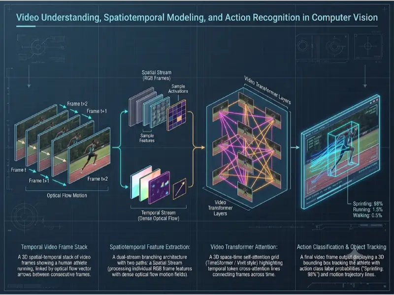
Applications range from autonomous driving trajectory prediction and sports performance analytics to industrial safety monitoring and AI video surveillance. Understanding how spatiotemporal representations evolve from classical differential motion fields to space-time self-attention transformers is essential for modern vision engineering.
Spatiotemporal Foundations & Optical Flow
The Temporal Dimension in Video Analysis
A video sequence is represented as a 4D tensor V ∈ &mathbb;RC × T × H × W, where C represents color channels, T specifies temporal frame count, and H × W denotes spatial image dimensions. Unlike static images where spatial correlation dominates, video streams exhibit high temporal redundancy between adjacent frames I(x, y, t) and I(x, y, t + Δt).
Optical Flow Estimation & Motion Dynamics
Optical flow quantifies two-dimensional vector motion fields [u(x, y), v(x, y)]T representing pixel displacement between consecutive video frames. The classical Brightness Constancy Constraint Equation assumes that pixel intensity remains constant along a motion trajectory:
$$
I(x, y, t) = I(x + \Delta x, y + \Delta y, t + \Delta t)
$$Applying a first-order Taylor series expansion yields the linear optical flow differential equation:
$$
\frac{\partial I}{\partial x} u + \frac{\partial I}{\partial y} v + \frac{\partial I}{\partial t} = 0 \quad \Rightarrow \quad I_x u + I_y v + I_t = 0
$$where Ix, Iy are spatial image gradients, It is temporal intensity derivative, and u = dx/dt, v = dy/dt are horizontal and vertical optical flow velocities.
Lucas-Kanade vs. Farnebäck Dense Optical Flow
- Lucas-Kanade Method (Sparse): Assumes constant local flow within a small W × W spatial window. Solves the overdetermined system using least-squares optimization to estimate velocity vectors at salient feature points (corners, edges).
- Farnebäck Method (Dense): Approximates local pixel neighborhoods using quadratic polynomial expansions, yielding smooth, dense motion vector fields across all pixels in a frame pair.
Interactive Quick Review: Brightness Constancy & Optical Flow
Test your understanding of temporal video representation and optical flow mechanics before exploring deep spatiotemporal architectures:
Quick Review Verification
1. What fundamental physical assumption underlies the Brightness Constancy Constraint in optical flow estimation?
Answer: It assumes that the observed brightness intensity of a surface point remains constant as it moves across adjacent video frames (I(x, y, t) = I(x + Δx, y + Δy, t + Δt)).
2. How does sparse optical flow (Lucas-Kanade) differ from dense optical flow (Farnebäck)?
Answer: Sparse optical flow calculates motion vectors only for specific salient feature points (e.g., corners), whereas dense optical flow estimates displacement vectors for every pixel in the frame.
Deep Spatiotemporal Architectures & Action Recognition
Two-Stream Convolutional Networks
Introduced by Simonyan and Zisserman, Two-Stream Networks decompose video understanding into separate spatial and temporal processing pathways:
- Spatial Stream ConvNet: Operates on static single RGB frames It to extract spatial scene context, object appearance, and background environment features.
- Temporal Stream ConvNet: Operates on stacked horizontal and vertical optical flow fields dt across L consecutive frames, isolating fine motion trajectory patterns independently of static appearance.
Class prediction scores from both streams are combined using late fusion (softmax averaging or SVM classification).
3D Convolutional Networks (C3D / I3D)
While standard 2D convolutions collapse temporal dimensions (KH × KW × C), 3D Convolutional Networks (C3D) convolve 3D filter kernels (KT × KH × KW) across spatial and temporal dimensions simultaneously:
$$
v_{ij}^{xyz} = \tanh \left( b_{ij} + \sum_{m} \sum_{p=0}^{P-1} \sum_{q=0}^{Q-1} \sum_{r=0}^{R-1} w_{ijm}^{pqr} v_{(i-1)m}^{(x+p)(y+q)(z+r)} \right)
$$Inflated 3D ConvNets (I3D): Addresses the lack of large-scale 3D pre-training datasets by inflating successful 2D ImageNet-pretrained architecture weights (e.g., Inception, ResNet) into 3D. A K × K 2D filter kernel is converted to a K × K × K 3D kernel by repeating the 2D weights K times along the temporal axis and scaling by 1/K to preserve activation response scales.
Video Transformers & Space-Time Self-Attention
Modern video models replace fixed-receptive-field 3D convolutions with global Transformer self-attention architectures.
Patch Tokenization in 3D Space-Time
A video tensor V ∈ &mathbb;RC × T × H × W is partitioned into non-overlapping 3D spatiotemporal tubelet patches of size PT × PH × PW. The total count of extracted space-time tokens N equals:
$$
N = \left( \frac{T}{P_T} \right) \times \left( \frac{H}{P_H} \right) \times \left( \frac{W}{P_W} \right)
$$Tokens are projected linearly into D-dimensional embeddings and augmented with 3D learnable positional encodings.
Divided Space-Time Self-Attention (TimeSformer)
Applying full self-attention across all N spatiotemporal tokens yields quadratic compute complexity O(N2), which is computationally prohibitive for long video clips. TimeSformer solves this by decoupling self-attention into separate spatial and temporal passes:
- Temporal Self-Attention: For each spatial location (h, w), self-attention is evaluated exclusively across tokens at identical spatial positions across all time steps T. Compute complexity: O((T/PT)2).
- Spatial Self-Attention: For each time step t, self-attention is evaluated across all spatial tokens within that frame. Compute complexity: O((H/PH × W/PW)2).
Divided space-time attention achieves equivalent classification performance to joint attention while reducing computational latency by an order of magnitude.
Multi-Object Tracking (MOT) & Trajectory Analysis
Action recognition often requires tracking individual moving entities across extended temporal sequences. The dominant paradigm is Tracking-by-Detection.
The Tracking-by-Detection Framework
- Object Detection: A 2D detector (YOLO / Faster R-CNN) identifies object bounding boxes in frame t.
- Motion Estimation (Kalman Filtering): Predicts bounding box spatial state x = [u, v, s, r, u˙, v˙, s˙]T in frame t + 1 using a linear constant-velocity state transition model.
- Data Association (Hungarian Algorithm): Matches predicted Kalman states against newly detected bounding boxes by solving a bipartite graph matching problem.
SORT vs. DeepSORT Architecture
- SORT (Simple Online and Realtime Tracking): Associates detections using spatial overlap via Intersection over Union (IoU) distances. Fast (>60 FPS), but prone to ID switches during target occlusions.
- DeepSORT: Augments IoU spatial distances with deep appearance feature embeddings extracted from a re-identification (Re-ID) neural network. Data association uses a weighted metric combining Mahalanobis motion distance d(1) and visual appearance cosine distance d(2):
Integrating visual embeddings allows DeepSORT to maintain object identities through extended occlusions and camera motion.
Architectural Comparison Matrix
The following table summarizes key technical trade-offs across video understanding architectures:
| Architecture / Paradigm | Temporal Modeling Mechanism | Computational Complexity | Key Strengths | Primary Limitations |
|---|---|---|---|---|
| Two-Stream CNNs | Explicit pre-computed optical flow | Moderate (High pre-process cost) | Strong explicit motion capture | Expensive optical flow pre-processing |
| 3D CNNs (C3D / I3D) | 3D spatial-temporal convolutions | High (O(KT · KH · KW)) | End-to-end spatiotemporal learning | Heavy FLOP load, short temporal window |
| TimeSformer (Divided Attention) | Decoupled space-time self-attention | Moderate (O(T2 + (HW)2)) | Captures long-range relationships | Requires large training datasets |
| DeepSORT Tracking | Kalman filter + Re-ID embeddings | Low / Real-Time (>30 FPS) | Resilient against object occlusions | Fails under heavy detector missed-detections |
Spatial Computing & Real-World Applications
Video understanding and action recognition power critical industrial and commercial systems:
- Autonomous Vehicle Behavior Prediction: Analyzing multi-camera video streams to track surrounding pedestrians and vehicles, predicting trajectory intents seconds into the future.
- Sports Performance Analytics: Tracking ball trajectories, player kinematics, and tactical formation movements in real time during high-speed athletic broadcasts.
- Industrial Workplace Safety Monitoring: Detecting hazardous personnel behaviors, heavy machinery compliance violations, or worker fall incidents in factory environments.
- Automated Video Indexing and Search: Tagging, searching, and summarizing thousands of hours of video content based on fine-grained action descriptions.
History, Challenges, and Future of Video Understanding
History and Evolution
Video analysis originated in the 1990s with classical hand-crafted motion descriptors like Space-Time Interest Points (STIP) and Improved Dense Trajectories (iDT). The deep learning era began with Two-Stream CNNs in 2014, followed by 3D Convolutional Networks (C3D/I3D) in 2017. Since 2021, Video Transformers (TimeSformer, ViViT) have redefined state-of-the-art benchmark performance by scaling space-time self-attention.
Current Technical & Operational Challenges
Deploying video models presents major technical constraints:
- Extreme Compute and Memory Footprint: Storing multi-frame feature maps during backpropagation rapidly consumes GPU memory bandwidth.
- Temporal Scale Ambiguity: Actions occur at drastically different speeds (e.g., a rapid blink vs. a slow gait cycle), requiring multi-scale temporal sampling rates.
- Camera Egomotion Distortion: Dynamic camera movement (handheld cameras, drone footage) introduces severe background optical flow that masks true foreground target motion.
- Long-Form Video Reasoning: Analyzing hours-long movies or surveillance streams requires memory architectures that extend beyond short 16-frame sampling windows.
Future Potentials & Emerging Paradigms
Future developments focus on Multimodal Video Foundation Models. Architectures like Video-LLaVA and Sora integrate video understanding with Large Language Models and diffusion generative frameworks, enabling natural language video Q&A, automated video generation, and agentic long-form reasoning.
Engineering Trade-offs
Engineering video analysis systems requires key architectural decisions:
- Dense Optical Flow vs. End-to-End Learning: Pre-computing optical flow guarantees explicit motion signals but introduces heavy CPU/GPU pre-processing latency, whereas 3D CNNs learn motion implicitly at higher compute costs.
- Frame Sampling Rate vs. Memory Footprint: Sampling frames at high frame rates (e.g., 60 fps) captures rapid motion but expands memory consumption, whereas sparse frame sampling risks temporal motion aliasing.
- Joint Space-Time Attention vs. Divided Space-Time Attention: Joint space-time attention models complex feature interactions across all tokens but scales quadratically (O(N2)), whereas divided attention drops compute complexity (O(T2 + S2)) with minimal accuracy loss.
Interactive Quick Review: TimeSformer & Tracking Trade-offs
Reinforce key concepts regarding video transformer tokenization and DeepSORT tracking mechanics before reviewing the FAQ:
Quick Review Verification
1. How does divided space-time attention reduce computational complexity in TimeSformer?
Answer: It decouples full 3D self-attention into two separate 1D passes: temporal self-attention across frames for identical spatial locations, followed by spatial self-attention within individual frames. This reduces complexity from quadratic O((S · T)2) to additive O(T2 + S2).
2. What specific disadvantage of SORT tracking is resolved by DeepSORT’s appearance embeddings?
Answer: SORT relies solely on bounding box spatial overlap (IoU), causing target identity switches (ID switches) during occlusions. DeepSORT incorporates deep visual appearance Re-ID embeddings to maintain correct object identities even after targets reappear from behind occlusions.
External References and Further Reading
To explore spatiotemporal architectures, video transformers, and multi-object tracking, consult the following authoritative sources:
- Two-Stream Convolutional Networks for Action Recognition in Videos (Simonyan & Zisserman, 2014) – The seminal research paper establishing dual spatial and temporal network pathways.
- Is Space-Time Attention All You Need for Video Understanding? (TimeSformer, Bertasius et al., 2021) – Official research paper introducing divided space-time self-attention for video transformers.
- DeepSORT: Simple Online and Realtime Tracking with a Deep Association Metric – Open-source repository and paper detailing Kalman filtering and appearance feature data association.
Frequently Asked Questions about Video Understanding and Action Recognition
Why is 3D convolution computationally more expensive than 2D convolution?
A 2D convolution slides a 2D filter kernel (KH × KW) across spatial height and width. A 3D convolution adds a temporal dimension, sliding a 3D filter volume (KT × KH × KW) across spatial coordinates and multiple temporal frame stacks. This multiplies multiplication-addition FLOP operations by the temporal kernel factor KT.
How does Inflated 3D ConvNet (I3D) leverage 2D ImageNet pre-trained weights?
Training 3D networks from scratch requires massive video datasets. I3D bootstrap-initializes 3D network weights by cloning 2D spatial weights W2D along the temporal dimension KT times, dividing each copied weight by KT (W3D = W2D / KT). This preserves pre-trained spatial feature detectors while enabling immediate 3D fine-tuning.
What is the function of the Kalman Filter in object tracking pipelines like SORT and DeepSORT?
The Kalman filter predicts an object’s future bounding box state (position, aspect ratio, velocity) in frame t+1 based on its motion history. This provides an estimated target location to correlate against new object detections, smoothing noisy trajectory estimates and maintaining tracking during brief detection misses.
Why is camera egomotion problematic for action recognition models?
Optical flow measures total pixel displacement on the image sensor. When the camera moves (panning, zooming, or mounted on a moving vehicle), background pixels experience massive optical flow displacements. This background motion noise drowns out the true relative motion of target subjects, degrading action classification unless background homography compensation is applied.
What is the difference between Tubelet Embedding and Frame-level Embedding in Video Transformers?
Frame-level embedding tokenizes individual 2D image frames independently into 2D spatial patches before concatenating tokens across time. Tubelet embedding tokenizes 3D space-time volumes (PT × PH × PW) directly, fusing spatial and temporal information inside the initial linear projection layer.
How does the Hungarian Algorithm resolve data association in DeepSORT?
The Hungarian algorithm is a combinatorial optimization algorithm that solves global maximum-bipartite matching in polynomial time O(N3). In DeepSORT, it takes a cost matrix containing combined spatial Mahalanobis distances and visual appearance distances between predicted Kalman tracks and new detector bounding boxes, computing the globally optimal track-to-detection assignment pair.
Why are long-term actions difficult to capture with standard 16-frame 3D CNNs?
Standard 16-frame clips sampled at 30 fps capture only 0.5 seconds of temporal context. Complex composite activities (e.g., “baking a cake” or “assembling an engine”) span several minutes. Capturing these long-range temporal dependencies requires hierarchical video transformers or long-term recurrent memory banks.
What is SlowFast Network architecture in action recognition?
SlowFast is a dual-pathway 3D CNN model inspired by biological vision. The Slow Pathway operates at a low frame rate with high channel capacity to capture detailed spatial appearance. The Fast Pathway operates at a high frame rate (refresh rate) with low channel capacity to capture fast motion dynamics efficiently.
End-of-Page Exercises: Review, Thought-Provoking & Engineering Problems
Review Questions and Answers
1. State the Brightness Constancy Constraint Equation in differential form.
Answer: Ix u + Iy v + It = 0, where Ix, Iy are spatial gradients, It is temporal intensity derivative, and u, v are optical flow velocity components.
2. What two processing streams make up a Two-Stream Convolutional Network?
Answer: The Spatial Stream (processing single RGB frames for appearance context) and the Temporal Stream (processing stacked optical flow vectors for motion context).
3. How are 2D filter weights scaled when inflated into 3D weights in the I3D architecture?
Answer: The 2D weights are repeated K times along the temporal dimension and divided by K (W3D = W2D / K) to preserve activation magnitudes.
4. Write the formula calculating total 3D space-time tokens N for a video tensor V given tubelet size PT × PH × PW.
Answer: N = (T / PT) × (H / PH) × (W / PW).
5. What two attention operations replace full 3D self-attention in the TimeSformer architecture?
Answer: Temporal Self-Attention (across time for identical spatial coordinates) and Spatial Self-Attention (across spatial coordinates within individual frames).
6. What algorithm is used for data association in SORT and DeepSORT multi-object tracking?
Answer: The Hungarian Algorithm (Munkres Algorithm) for solving bipartite graph matching.
7. What state vector variables are tracked by a linear Kalman filter in standard bounding box tracking?
Answer: x = [u, v, s, r, u˙, v˙, s˙]T, representing center coordinates (u, v), scale area s, aspect ratio r, and corresponding velocities.
8. What metric distance does SORT use to measure bounding box similarity between frames?
Answer: Intersection over Union (IoU) spatial distance.
9. What extra metric component does DeepSORT combine with motion distance for tracking data association?
Answer: Deep visual appearance cosine distance extracted from a deep Re-ID neural network.
10. Name four major real-world application domains for video understanding models.
Answer: Autonomous driving behavior prediction, sports kinematics analytics, industrial safety monitoring, and automated video search indexing.
Thought-Provoking Questions and Answers
1. Why does a single-stream 2D CNN trained on individual RGB frames often achieve surprisingly high accuracy on action recognition benchmarks like UCF101?
Answer: Many action recognition datasets contain strong static background bias (scene context shortcuts). For instance, an image containing a swimming pool strongly correlates with “swimming” regardless of motion dynamics, allowing single-frame 2D CNNs to exploit spatial context without learning true temporal motion patterns.
2. How does the aperture problem create ambiguity when estimating local optical flow using differential gradient operators?
Answer: When viewed through a small local aperture, motion along a straight edge line is ambiguous; only the velocity component orthogonal to the edge direction can be measured (Ix u + Iy v = –It). Motion parallel to the edge produces zero spatial derivative change, requiring corner features or spatial neighborhood constraints (Lucas-Kanade window) to resolve true 2D velocity vectors.
3. Why does divided space-time attention in TimeSformer maintain high action classification accuracy while drastically reducing computational FLOPs?
Answer: Video motion displays strong structural factorization: spatial appearance structures move continuously along smooth temporal trajectories. Decoupling spatial attention (learning “what” objects look like) from temporal attention (learning “how” objects move) mirrors this factorized physical reality, removing redundant cross-token comparisons across distant space-time points.
4. How does target occlusion cause SORT tracking pipelines to create high numbers of false ID switches?
Answer: SORT relies strictly on overlapping bounding boxes (IoU). When a tracked target is occluded behind another object or pole for several frames, no detector bounding box overlaps the Kalman predicted track. The track is deleted after max-age expiration. When the target emerges, SORT assigns it a brand-new track ID, causing an ID switch error.
5. Why is temporal sampling stride selection critical when processing high frame-rate sports footage (e.g., 120 FPS)?
Answer: At 120 FPS, adjacent frames exhibit minimal pixel displacement. If a 16-frame 3D CNN samples consecutive frames without temporal stride (s = 1), the total temporal receptive field spans only 0.13 seconds, missing complete human movement phases. Applying a temporal stride (e.g., s = 4 or s = 8) expands the effective temporal window to capture full gait cycles and kinetic actions.
6. How do optical flow inputs make Two-Stream CNNs more robust against background texture overfitting than pure 3D CNNs?
Answer: Pre-computed optical flow isolates motion vectors (u, v) while discarding static color textures, lighting variations, and background visual identity. The temporal stream network is forced to learn pure motion geometry (e.g., rotational velocity, trajectory curvature) without shortcutting to spatial background cues.
7. In what scenario would a linear constant-velocity Kalman filter fail in an autonomous driving tracking pipeline?
Answer: Linear constant-velocity Kalman filters assume objects move in straight paths at steady speeds. If an oncoming vehicle executes an abrupt emergency turn or hard braking maneuver, the linear state prediction deviates severely from actual detector measurements, causing bounding box assignment mismatches in the Hungarian matcher.
8. How does tubelet embedding differ structurally from standard 2D patch tokenization in video transformers?
Answer: 2D patch tokenization slices individual frames independently into flat 2D spatial patches (PH × PW). Tubelet embedding projects 3D spatiotemporal volumes (PT × PH × PW) directly using 3D linear projections, fusing dynamic motion and spatial appearance into token representations right at the input layer.
9. Why do dynamic camera movements (e.g., drone camera panning) degrade action recognition models?
Answer: Drone camera panning induces global optical flow across the entire background matrix. The temporal network receives heavy background motion signals that conceal relative foreground subject motion, causing misclassifications unless homography registration is used to cancel global camera rotation.
10. How do multimodal generative video foundation models (e.g., Sora) perform spatial-temporal reasoning differently from classification CNNs?
Answer: Classification CNNs compress 4D video tensors down to scalar class probability distributions. Diffusion video foundation models learn a generative latent spatial-temporal representation that models physical dynamics, object persistence, 3D geometry consistency, and light transport over time, enabling dynamic video synthesis and predictive simulation.
Numerical Engineering Problems & Solutions
Problem 1: Optical Flow Velocity Calculation
In a video stream, spatial intensity gradients at pixel coordinate (100, 150) are evaluated as Ix = 4.0 and Iy = -3.0 gray levels/pixel. The temporal intensity derivative between consecutive frames is It = 12.0 gray levels/frame. Assuming horizontal motion velocity component u = 1.50 pixels/frame, evaluate vertical optical flow velocity v in pixels/frame using the Brightness Constancy Constraint Equation.
In a video stream, spatial intensity gradients at pixel coordinate (100, 150) are evaluated as Ix = 4.0 and Iy = -3.0 gray levels/pixel. The temporal intensity derivative between consecutive frames is It = 12.0 gray levels/frame. Assuming horizontal motion velocity component u = 1.50 pixels/frame, evaluate vertical optical flow velocity v in pixels/frame using the Brightness Constancy Constraint Equation.
Solution:
- Brightness Constancy Equation: Ix u + Iy v + It = 0.
- Substitute known values: (4.0 × 1.50) + (-3.0 × v) + 12.0 = 0.
- Simplify: 6.0 – 3.0v + 12.0 = 0 &implies; 18.0 = 3.0v.
- Solve for v: v = 18.0 / 3.0 = 6.0 pixels/frame.
Answer: Vertical optical flow velocity component is v = +6.0 pixels/frame.
Problem 2: 3D Convolution FLOP Count Comparison
A standard 2D convolution layer applies 64 filter kernels of size 3×3 across a 224 × 224 feature map with 3 input channels. A 3D convolution layer applies 64 filter kernels of size 3×3×3 (temporal kernel size KT = 3) across a 16-frame 224 × 224 video stack with 3 input channels. Calculate FLOPs per frame for both layers (excluding bias) and determine computational expansion factor of 3D over 2D convolution.
A standard 2D convolution layer applies 64 filter kernels of size 3×3 across a 224 × 224 feature map with 3 input channels. A 3D convolution layer applies 64 filter kernels of size 3×3×3 (temporal kernel size KT = 3) across a 16-frame 224 × 224 video stack with 3 input channels. Calculate FLOPs per frame for both layers (excluding bias) and determine computational expansion factor of 3D over 2D convolution.
Solution:
- 2D Conv FLOPs (single frame): 224 × 224 × 3 × (3 × 3) × 64 × 2 = 173,408,256 FLOPs (~173.41 MFLOPs).
- 3D Conv FLOPs (16 frames): 16 × 224 × 224 × 3 × (3 × 3 × 3) × 64 × 2 = 8,323,596,288 FLOPs (~8,323.60 MFLOPs).
- Per-frame 3D Conv FLOPs: 8,323,596,288 / 16 = 520,224,768 FLOPs (~520.22 MFLOPs).
- Expansion factor per frame: 520.22 / 173.41 = 3.0× (equals temporal kernel size KT = 3). Total clip FLOP expansion = 16 × 3 = 48.0×.
Answer: 2D layer requires 173.41 MFLOPs/frame; 3D layer requires 520.22 MFLOPs/frame (3.0× per-frame expansion factor; 48× total clip expansion).
Problem 3: Video Transformer Token Count Calculation
A high-definition video clip tensor V has temporal duration T = 32 frames and spatial resolution H = 224 pixels, W = 224 pixels. A TimeSformer model processes the video using 3D tubelet patches of size PT = 2 frames, PH = 16 pixels, PW = 16 pixels. Calculate total space-time token count N generated for Transformer self-attention.
A high-definition video clip tensor V has temporal duration T = 32 frames and spatial resolution H = 224 pixels, W = 224 pixels. A TimeSformer model processes the video using 3D tubelet patches of size PT = 2 frames, PH = 16 pixels, PW = 16 pixels. Calculate total space-time token count N generated for Transformer self-attention.
Solution:
- Temporal tokens: NT = T / PT = 32 / 2 = 16 temporal steps.
- Spatial tokens per frame: NS = (H / PH) × (W / PW) = (224 / 16) × (224 / 16) = 14 × 14 = 196 spatial tokens.
- Total 3D tokens: N = NT × NS = 16 × 196 = 3,136 spatiotemporal tokens.
Answer: Video clip generates 3,136 spatiotemporal tokens.
Problem 4: Self-Attention Compute Complexity Comparison
For a token sequence of length N = 3,136 (from Problem 3 with NT = 16 temporal tokens and NS = 196 spatial tokens), calculate scalar self-attention dot-product operations (N2) for: (a) Full Joint Space-Time Self-Attention, and (b) Divided Space-Time Self-Attention (Temporal attention pass + Spatial attention pass). Calculate computational reduction factor achieved by divided attention.
For a token sequence of length N = 3,136 (from Problem 3 with NT = 16 temporal tokens and NS = 196 spatial tokens), calculate scalar self-attention dot-product operations (N2) for: (a) Full Joint Space-Time Self-Attention, and (b) Divided Space-Time Self-Attention (Temporal attention pass + Spatial attention pass). Calculate computational reduction factor achieved by divided attention.
Solution:
- Full Joint Attention ops: N2 = (3136)2 = 9,834,496 operations (~9.83 million).
- Divided Temporal Attention ops: NS × (NT)2 = 196 × (16)2 = 196 × 256 = 50,176 ops.
- Divided Spatial Attention ops: NT × (NS)2 = 16 × (196)2 = 16 × 38,416 = 614,656 ops.
- Total Divided Attention ops: 50,176 + 614,656 = 664,832 operations (~0.665 million).
- Reduction factor: 9,834,496 / 664,832 ≈ 14.79× compute reduction.
Answer: Joint attention requires 9.83M ops; divided attention requires 0.665M ops (a 14.79× computational reduction factor).
Problem 5: Optical Flow Frame Storage Memory Footprint
A high-speed industrial camera captures 1080p video (1920 × 1080 pixels) at 60 FPS. Dense optical flow fields store horizontal u and vertical v displacement vectors as 32-bit (4-byte) single-precision floats per pixel. Calculate memory required to store uncompressed optical flow for a 10-second video clip in Megabytes (MB). (1 MB = 106 bytes).
A high-speed industrial camera captures 1080p video (1920 × 1080 pixels) at 60 FPS. Dense optical flow fields store horizontal u and vertical v displacement vectors as 32-bit (4-byte) single-precision floats per pixel. Calculate memory required to store uncompressed optical flow for a 10-second video clip in Megabytes (MB). (1 MB = 106 bytes).
Solution:
- Total frames in 10 seconds: 10 × 60 = 600 frames (599 optical flow field pairs).
- Bytes per optical flow frame pair: 1920 × 1080 pixels × 2 channels (u, v) × 4 bytes/float = 16,588,800 bytes (~16.59 MB/frame).
- Total clip storage: 599 optical flow pairs × 16,588,800 bytes = 9,936,691,200 bytes = 9,936.69 MB (~9.94 Gigabytes).
Answer: Storing uncompressed optical flow for 10 seconds requires 9,936.69 MB (~9.94 GB).
Problem 6: Bounding Box IoU Calculation for SORT Tracking
In frame t + 1, a Kalman filter predicts a target bounding box Bpred with coordinates [x1, y1, x2, y2] = [100, 100, 200, 200] (area 100 × 100 = 10,000 pixels2). An object detector detects bounding box Bdet = [150, 100, 250, 200] (area 100 × 100 = 10,000 pixels2). Calculate intersection box area, union box area, and evaluate Intersection over Union (IoU) spatial match score.
In frame t + 1, a Kalman filter predicts a target bounding box Bpred with coordinates [x1, y1, x2, y2] = [100, 100, 200, 200] (area 100 × 100 = 10,000 pixels2). An object detector detects bounding box Bdet = [150, 100, 250, 200] (area 100 × 100 = 10,000 pixels2). Calculate intersection box area, union box area, and evaluate Intersection over Union (IoU) spatial match score.
Solution:
- Intersection box coordinates: [max(100,150), max(100,100), min(200,250), min(200,200)] = [150, 100, 200, 200].
- Intersection dimensions: Width = 200 – 150 = 50; Height = 200 – 100 = 100. Intersection Area = 50 × 100 = 5,000 pixels2.
- Union Area = Area(Bpred) + Area(Bdet) – Intersection Area = 10,000 + 10,000 – 5,000 = 15,000 pixels2.
- IoU score = Intersection / Union = 5,000 / 15,000 = 0.3333 (~33.33%).
Answer: Intersection over Union match score is IoU = 0.333 (33.3%).
Problem 7: DeepSORT Weighted Association Cost Metric
During track association, a target track i and detection j have evaluated Mahalanobis motion distance d(1) = 4.0 and deep appearance visual distance d(2) = 0.15. DeepSORT evaluates combined cost cij = λ d(1) + (1 – λ) d(2) with motion weighting hyperparameter λ = 0.10. Evaluate total matching cost cij.
During track association, a target track i and detection j have evaluated Mahalanobis motion distance d(1) = 4.0 and deep appearance visual distance d(2) = 0.15. DeepSORT evaluates combined cost cij = λ d(1) + (1 – λ) d(2) with motion weighting hyperparameter λ = 0.10. Evaluate total matching cost cij.
Solution:
- Motion cost term: λ d(1) = 0.10 × 4.0 = 0.40.
- Appearance cost term: (1 – 0.10) d(2) = 0.90 × 0.15 = 0.135.
- Combined cost cij = 0.40 + 0.135 = 0.535.
Answer: Total association matching cost is cij = 0.535.
Problem 8: Temporal Receptive Field Coverage Calculation
A 3D CNN model consists of 5 cascaded 3D convolution layers, each using temporal kernel size KT = 3 with zero temporal padding. Calculate total temporal receptive field span in frames. If the video is captured at 30 FPS, evaluate temporal receptive field duration in seconds.
A 3D CNN model consists of 5 cascaded 3D convolution layers, each using temporal kernel size KT = 3 with zero temporal padding. Calculate total temporal receptive field span in frames. If the video is captured at 30 FPS, evaluate temporal receptive field duration in seconds.
Solution:
- Receptive field calculation for L layers: RF = 1 + ∑i=1L (KT,i – 1) = 1 + 5 × (3 – 1) = 1 + 10 = 11 frames.
- Duration at 30 FPS: 11 / 30 = 0.3667 seconds (~366.7 ms).
Answer: Receptive field spans 11 frames (0.367 seconds).
Problem 9: SlowFast Network Frame Sampling Rates
A SlowFast network processes a 64-frame video clip sampled at 30 FPS (duration 2.133 seconds). The Slow Pathway samples frames using temporal stride τ = 8. The Fast Pathway samples frames using temporal stride τ/8 = 1. Calculate frame count processed by the Slow Pathway and Fast Pathway.
A SlowFast network processes a 64-frame video clip sampled at 30 FPS (duration 2.133 seconds). The Slow Pathway samples frames using temporal stride τ = 8. The Fast Pathway samples frames using temporal stride τ/8 = 1. Calculate frame count processed by the Slow Pathway and Fast Pathway.
Solution:
- Slow Pathway frame count: 64 / τ = 64 / 8 = 8 frames.
- Fast Pathway frame count: 64 / 1 = 64 frames.
Answer: Slow Pathway processes 8 frames; Fast Pathway processes 64 frames.
Problem 10: Hungarian Matching Cost Matrix Sizing
In an automated highway monitoring system, an object tracker maintains M = 25 active vehicle Kalman trajectories. A YOLOv8 detector outputs N = 35 new vehicle bounding boxes in frame t. Calculate size of bipartite assignment cost matrix passed to the Hungarian algorithm. Compute worst-case algorithmic complexity O(K3) where K = max(M, N).
In an automated highway monitoring system, an object tracker maintains M = 25 active vehicle Kalman trajectories. A YOLOv8 detector outputs N = 35 new vehicle bounding boxes in frame t. Calculate size of bipartite assignment cost matrix passed to the Hungarian algorithm. Compute worst-case algorithmic complexity O(K3) where K = max(M, N).
Solution:
- Cost matrix dimension: M × N = 25 × 35 entries (875 distance comparisons).
- Max dimension K = max(25, 35) = 35.
- Worst-case Hungarian complexity: K3 = (35)3 = 42,875 operations.
Answer: Cost matrix dimension is 25 × 35; worst-case matching complexity requires 42,875 operations.
Problem 11: Real-Time Execution Latency Budget
An autonomous robot vision system must perform action recognition and tracking at 30 FPS (total latency budget 33.33 ms/frame). The vision pipeline consists of four sequential stages: (1) Frame Capture & Preprocessing (3.5 ms), (2) Object Detection (14.0 ms), (3) DeepSORT Data Association (4.2 ms), and (4) Action Classifier Inference (10.5 ms). Calculate total pipeline latency and determine whether the system meets the 30 FPS real-time constraint.
An autonomous robot vision system must perform action recognition and tracking at 30 FPS (total latency budget 33.33 ms/frame). The vision pipeline consists of four sequential stages: (1) Frame Capture & Preprocessing (3.5 ms), (2) Object Detection (14.0 ms), (3) DeepSORT Data Association (4.2 ms), and (4) Action Classifier Inference (10.5 ms). Calculate total pipeline latency and determine whether the system meets the 30 FPS real-time constraint.
Solution:
- Total pipeline latency = 3.5 + 14.0 + 4.2 + 10.5 = 32.20 ms.
- Compare against 30 FPS target budget: 32.20 ms ≤ 33.33 ms.
- Equivalent frame rate: 1000 / 32.20 ≈ 31.05 FPS.
Answer: Total latency is 32.20 ms (~31.05 FPS), which successfully meets the 30 FPS real-time constraint.
Problem 12: I3D Inflation Weight Parameter Conservation
A 2D convolutional filter in a ResNet architecture has weight tensor W2D ∈ &mathbb;R64 × 32 × 7 × 7 (100,352 parameters). The filter is inflated into a 3D kernel with temporal kernel size KT = 7. Calculate total parameter count of the inflated 3D kernel W3D and evaluate memory expansion factor.
A 2D convolutional filter in a ResNet architecture has weight tensor W2D ∈ &mathbb;R64 × 32 × 7 × 7 (100,352 parameters). The filter is inflated into a 3D kernel with temporal kernel size KT = 7. Calculate total parameter count of the inflated 3D kernel W3D and evaluate memory expansion factor.
Solution:
- 2D parameter count: 64 × 32 × 7 × 7 = 100,352 float parameters.
- 3D parameter count: 64 × 32 × 7 × 7 × 7 = 702,464 float parameters.
- Expansion factor: 702,464 / 100,352 = 7.0× (equals temporal kernel length KT = 7).
Answer: Inflated 3D weight tensor contains 702,464 parameters (a 7.0× parameter expansion factor).
Video Understanding and Action Recognition — Summary & Wrap-Up
Video understanding algorithms extend computer vision into the temporal dimension. By evolving from classical brightness constancy optical flow fields (Ix u + Iy v + It = 0) and Two-Stream CNNs to 3D Inflated ConvNets (I3D), Divided Space-Time Attention Transformers (TimeSformer), and DeepSORT multi-object tracking pipelines (cij = λ d(1) + (1-λ) d(2)), modern video vision models analyze kinetic motion trajectories, track target identities, and predict complex human behaviors across real-time video streams.
Explore the Modern Computer Vision Sub-Cluster
Temporal video analysis forms a core pillar of modern visual intelligence. To explore spatial filtering, multi-view 3D geometry, and deep vision foundation models, navigate the complete sub-cluster:
3D Vision and Gaussian Splatting
Details multi-view geometry, pinhole camera projection, NeRF volume rendering, and real-time 3D Gaussian Splatting rasterization.
Digital Image Processing and 2D Analysis
Details classical spatial filtering, mathematical morphology, contrast enhancement, image compression file formats, and 2D biometric pattern recognition.
Video Understanding and Action Recognition
This page details spatiotemporal modeling, optical flow, video transformer architectures (TimeSformer), and real-time multi-object tracking across video streams.
Vision Transformers and Foundation Models
Explores modern deep learning vision architectures, patch tokenization in Vision Transformers (ViTs), DETR object detection, CLIP multimodal embedding, and zero-shot visual transfer.