
Swarm and multi-agent robotics studies how large groups of relatively simple autonomous robots coordinate their local actions to achieve complex collective behaviors. Rather than relying on a single monolithic controller, swarm architectures distribute sensing, computation, and decision-making across dozens, hundreds, or thousands of interacting agents.
This decentralized architecture allows multi-robot networks to operate robustly in communication-degraded or hostile environments where centralized infrastructure would introduce unacceptable latency or single points of failure. By exchanging localized states with immediate spatial neighbors, each robot executes deterministic update laws. When these interaction kernels are rigorously synthesized, globally coherent group behaviors emerge spontaneously.
The foundational challenge of swarm robotics lies in inverse synthesis: how can local microscopic interaction rules be mathematically guaranteed to produce desired macroscopic group behaviors? Tools from algebraic graph theory, distributed Lyapunov control, dynamic consensus, and non-convex optimization establish the analytical foundation for answering this question.
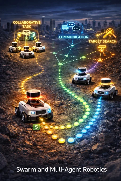
Decentralized spatial coordination: autonomous agents update local heading and velocity vectors using state information exchanged over dynamic peer-to-peer wireless communication graphs.
Swarm Intelligence Principles
In a robotic swarm, agents operate concurrently while communicating exclusively within a bounded wireless or optical neighborhood. No individual robot maintains a global map or centralized state vector. Collective capabilities—such as cooperative perimeter monitoring, distributed payload manipulation, and adaptive spatial foraging—emerge through iterative dynamic coupling across the network graph.
Interactive Quick Review: Decentralization & Local Interactions
Verify your understanding of decentralized architectures before examining graph theory and consensus matrices:
1. What is the fundamental inverse synthesis challenge in swarm and multi-agent robotics?
2. Why do decentralized multi-agent networks scale better than centralized master-slave architectures?
Network Representation and Algebraic Graph Theory
A multi-agent network is modeled as a time-varying graph:
$$ \mathcal{G}(t) = (\mathcal{V}, \mathcal{E}(t)) $$where:
- \(\mathcal{V} = \{v_1, v_2, \dots, v_N\}\): the vertex set representing \(N\) robotic agents
- \(\mathcal{E}(t) \subseteq \mathcal{V} \times \mathcal{V}\): the dynamic edge set representing active communication or sensing links
If agent \(i\) can receive transmissions from agent \(j\) at time \(t\), the directed edge \((v_j, v_i) \in \mathcal{E}(t)\). The open neighborhood \(\mathcal{N}_i(t)\) of agent \(i\) represents the set of peers directly influencing its local controller:
$$ \mathcal{N}_i(t) = \{ v_j \in \mathcal{V} \mid (v_j, v_i) \in \mathcal{E}(t) \} $$Dynamic Consensus Algorithms
Consensus protocols enable distributed agents to converge to a shared state value (e.g., orientation, rendezvous position, or environmental parameter estimate) exclusively through local peer exchanges.
In discrete time, each agent \(i\) updates its continuous state \(x_i \in \mathbb{R}^d\) according to the convex combination:
$$ x_i(t+1) = \sum_{j \in \mathcal{N}_i(t) \cup \{i\}} w_{ij}(t) \, x_j(t) $$where the coupling weights \(w_{ij}\) satisfy the row-stochastic property:
$$ w_{ij} \ge 0, \quad \sum_{j} w_{ij} = 1 \quad \forall i $$When the communication network is undirected and weight matrices are doubly stochastic (\(\sum_i w_{ij} = 1\)), the network converges asymptotically to the exact arithmetic average of initial states:
$$ \lim_{t \to \infty} x_i(t) = \frac{1}{N} \sum_{k=1}^N x_k(0) $$Graph Laplacian and Network Stability
The convergence dynamics of multi-agent networks are determined by the spectral properties of the Graph Laplacian matrix \(\mathbf{L}\).
For an unweighted, undirected graph \(\mathcal{G}\), let \(\mathbf{A} \in \mathbb{R}^{N \times N}\) denote the symmetric adjacency matrix, where \(A_{ij} = 1\) if \((i, j) \in \mathcal{E}\) and \(0\) otherwise. The diagonal degree matrix \(\mathbf{D}\) is given by:
$$ D_{ii} = \sum_{j=1}^N A_{ij} = |\mathcal{N}_i| $$The graph Laplacian \(\mathbf{L}\) is defined as:
$$ \mathbf{L} = \mathbf{D} - \mathbf{A} $$In continuous time, linear consensus dynamics follow the system of differential equations:
$$ \dot{\mathbf{x}}(t) = -\mathbf{L} \mathbf{x}(t) $$Because all row sums of \(\mathbf{L}\) equal zero, \(\mathbf{L}\mathbf{1}_N = \mathbf{0}\), establishing that the smallest eigenvalue is always \(\lambda_1 = 0\) with corresponding eigenvector \(\mathbf{1}_N = [1, 1, \dots, 1]^T\). For a connected undirected graph, the eigenvalues satisfy:
$$ 0 = \lambda_1 < \lambda_2 \le \lambda_3 \le \dots \le \lambda_N $$The second-smallest eigenvalue \(\lambda_2(\mathbf{L})\) is the algebraic connectivity (Fiedler value). It dictates the worst-case asymptotic convergence rate of the consensus protocol:
$$ \|\mathbf{x}(t) - x_{\text{consensus}} \mathbf{1}_N\| \le e^{-\lambda_2(\mathbf{L}) t} \|\mathbf{x}(0) - x_{\text{consensus}} \mathbf{1}_N\| $$Formation Control and Leader–Follower Dynamics
Formation control maintains specified inter-agent geometric displacements \(\mathbf{d}_{ij} = \mathbf{p}_i^* - \mathbf{p}_j^*\) while navigating spatial domains.
For holonomic kinematic agents with positions \(\mathbf{p}_i \in \mathbb{R}^2\), a continuous formation stabilization control law is formulated as:
$$ \dot{\mathbf{p}}_i = -\sum_{j \in \mathcal{N}_i} \left[ (\mathbf{p}_i - \mathbf{p}_j) - \mathbf{d}_{ij} \right] $$In Leader–Follower architectures, one or more agents track an external target trajectory \(\mathbf{p}_L(t)\). Follower dynamics incorporate an additional pinning gain \(\kappa_i > 0\):
$$ \dot{\mathbf{p}}_i = -\sum_{j \in \mathcal{N}_i} (\mathbf{p}_i - \mathbf{p}_j - \mathbf{d}_{ij}) - \kappa_i (\mathbf{p}_i - \mathbf{p}_L - \mathbf{d}_{iL}) $$Distributed Convex Optimization
Robotic swarms cooperatively solve large-scale parameter estimation and resource allocation tasks without central aggregation. Let each agent hold a private local convex objective function \(f_i: \mathbb{R}^d \to \mathbb{R}\). The collective optimization problem is:
$$ \min_{\mathbf{x} \in \mathbb{R}^d} \sum_{i=1}^N f_i(\mathbf{x}) $$Under the Distributed Subgradient Method (DSM), each robot executes a combined consensus mixing and local gradient descent step:
$$ \mathbf{x}_i(t+1) = \sum_{j \in \mathcal{N}_i} w_{ij} \mathbf{x}_j(t) - \alpha(t) \nabla f_i(\mathbf{x}_i(t)) $$where \(\alpha(t) > 0\) represents a diminishing step-size schedule satisfying \(\sum_t \alpha(t) = \infty\) and \(\sum_t \alpha^2(t) < \infty\).
Contemporary 2026 AI-Era Formulations: MARL and Neural Solvers
Modern swarm robotics bridges classical algebraic graph consensus with distributed machine learning to handle non-linear dynamics, intermittent communication, and adversarial environments.
1. Multi-Agent Reinforcement Learning (MARL)
Using the Centralized Training with Decentralized Execution (CTDE) paradigm—exemplified by Multi-Agent PPO (MAPPO) and QMIX—agents optimize individual actor policies \(\pi_{\theta_i}(a_i \mid o_i)\) conditioned strictly on local sensor observations \(o_i\). A centralized critic guides training offline by observing joint state-action pairs, eliminating communication overhead during runtime deployment.
2. Decentralized Physics-Informed Neural Networks (Dec-PINNs)
When swarms map continuous spatiotemporal physical fields (e.g., thermal plumes, atmospheric pollution, ocean currents), agents utilize Dec-PINNs. Each robot maintains a compact neural surrogate parameterized by weights \(\boldsymbol{\theta}_i\) regularized by physical partial differential equations (such as advection-diffusion-reaction equations):
$$ \mathcal{L}_i(\boldsymbol{\theta}_i) = \mathcal{L}_{\text{sensor}}(\boldsymbol{\theta}_i) + \lambda_{\text{pde}} \left\| \frac{\partial u_i}{\partial t} + \mathbf{v} \cdot \nabla u_i - D \nabla^2 u_i \right\|^2 + \beta \sum_{j \in \mathcal{N}_i} \|\boldsymbol{\theta}_i - \boldsymbol{\theta}_j\|^2 $$The consensus regularization term \(\beta \sum \|\boldsymbol{\theta}_i - \boldsymbol{\theta}_j\|^2\) synchronizes neural weights across local wireless links, producing unified global field reconstructions without centralized data harvesting.
Operational Challenges and Failure Modes
- Wireless Channel Saturation & Packet Drop: High-density broadcast environments experience severe radio-frequency packet collisions, which breaks the row-stochasticity of consensus weight matrices.
- Byzantine & Malicious Agents: Compromised agents transmitting falsified state information can pull standard linear consensus algorithms away from equilibrium. Robust networks implement Fault-Tolerant Consensus (e.g., Mean-Subsequence-Reduced algorithms).
- Emergent Deadlocks: Artificial potential fields frequently produce local minima where attractive goal forces and neighbor repulsive vectors cancel out, trapping groups in deadlock formations.
- Hardware Heterogeneity & Sensor Drift: Discrepancies in wheel slip, battery degradation, and IMU biases cause uncalibrated swarm formations to skew over extended operational cycles.
Interactive Quick Review: Spectral Graph Theory & Optimization
Test your comprehension of graph Laplacians, algebraic connectivity, and distributed updates before reading the FAQ:
1. What is the physical significance of the algebraic connectivity \(\lambda_2(\mathbf{L})\) in consensus networks?
2. How does the row-stochastic weight condition guarantee consensus stability?
External References and Further Reading
Consult the following peer-reviewed resources for advanced study in multi-agent control and swarm theory:
- Flocking, Swarming, and Schooling (Couzin et al.) – Seminal biological foundations of self-organizing collective animal motion.
- IEEE Transactions on Automatic Control – Premier journal publishing rigorous theoretical proofs on consensus stability, Laplacian spectra, and distributed filtering.
- Harvard Wyss Institute Kilobot Project – Experimental testbed demonstrating collective shape formation across swarms of over 1,000 physical robots.
Frequently Asked Questions about Swarm and Multi-Agent Robotics
What differentiates a robot swarm from a conventional multi-robot system (MRS)?
A robot swarm consists of high-density populations (tens to thousands) of relatively simple, homogeneous agents relying strictly on local decentralized sensing without central coordination. An MRS often comprises smaller teams of heterogeneous, highly capable robots utilizing structured task assignment and direct point-to-point communication.
How does algebraic connectivity \(\lambda_2\) affect real-world drone swarms?
Algebraic connectivity measures network communication robustness. In aerial drone swarms operating under RF path loss, a low \(\lambda_2\) value indicates a bottleneck link where packet drops can split the swarm into isolated, uncoordinated clusters.
How do swarms avoid inter-agent collisions without global trajectory planners?
Agents evaluate local artificial potential fields or Control Barrier Functions (CBFs). Repulsive potential gradients generate steering vectors that push agents away from neighbors when distances drop below a safety radius \(d_{\text{safe}}\).
What are the industrial deployment domains for multi-agent swarm platforms?
Primary commercial deployments include automated warehouse parcel sorting (Automated Guided Vehicles / Autonomous Mobile Robots), precision agricultural crop spraying, environmental ocean monitoring, and post-disaster structural search and rescue.
How does leader–follower tracking balance formation shape against path tracking?
Followers combine consensus-based inter-agent displacement errors with proportional trajectory errors directed at virtual leaders. Adjusting the relative gains allows system engineers to prioritize rigid formation geometry versus rapid path tracking.
How do Byzantine fault tolerance protocols neutralize rogue agents?
In Mean-Subsequence-Reduced (MSR) consensus protocols, each robot gathers state reports from its neighborhood, eliminates the \(F\) highest and \(F\) lowest outlier values, and computes its state update strictly from the remaining values, neutralizing up to \(F\) faulty or malicious nodes.
What academic subjects provide the foundation for multi-agent systems engineering?
Key foundational disciplines include algebraic graph theory, linear algebra and matrix perturbation theory, Lyapunov stability analysis, distributed optimization, and multi-agent reinforcement learning.
End-of-Page Exercises: Review, Conceptual Analysis & Derivations
Part I: Review Questions
1. How is a multi-agent robotic network represented mathematically in algebraic graph theory?
2. State the discrete-time update rule governing linear consensus across connected neighbors.
3. How is the graph Laplacian matrix \(\mathbf{L}\) computed from degree matrix \(\mathbf{D}\) and adjacency matrix \(\mathbf{A}\)?
4. What spectral property of the Laplacian matrix corresponds to network algebraic connectivity?
5. Write the differential equation governing formation stabilization between kinematic agents.
6. State the continuous follower dynamics in a basic leader–follower tracking architecture.
7. What global optimization problem is solved via distributed consensus optimization?
8. List four major applications of autonomous multi-agent robotics.
9. Name four operational failure modes in decentralized physical robot swarms.
10. List five mathematical and engineering disciplines required for advanced swarm research.
Part II: Thought-Provoking Conceptual Questions
1. Why does decentralized local interaction prevent catastrophic single-point failures?
2. How does algebraic connectivity \(\lambda_2(\mathbf{L})\) dictate formation stability under high-rate wireless packet drop?
3. What physical constraints emerge when scaling distributed algorithms from 10 to 10,000 agents?
4. How do artificial potential fields generate local minimum deadlocks in multi-agent path planning?
5. Why is macro-level emergence difficult to engineer deterministically from micro-level rules?
6. In what scenarios do heterogeneous multi-robot systems outperform homogeneous swarms?
7. How do Byzantine fault-tolerant consensus protocols protect swarms against malicious agents?
8. Why do distributed optimization algorithms require symmetric communication graph topologies?
9. What role does stigmergy play in bio-inspired robotic coordination?
10. How does asymmetric packet loss break the row-stochastic property of consensus update matrices?
11. Why is continuous self-calibration vital in educational and research swarm deployments?
12. What economic and operational advantages do reconfigurable modular swarms offer over single monolithic robots?
Part III: Step-by-Step Numerical Engineering Derivations
Problem 1: Exact Average Consensus in a Complete Graph
Scenario: Three cooperative robots start with initial scalar estimates \(x_1(0) = 5.0 \text{ m}\), \(x_2(0) = 11.0 \text{ m}\), and \(x_3(0) = 20.0 \text{ m}\). In a complete communication graph (\(\mathcal{K}_3\)), all agents exchange values using uniform weights \(w_{ij} = 1/3\). Compute the updated state \(x_i(1)\) after one consensus iteration.
Step-by-Step Derivation:
$$ \begin{aligned} x_i(1) &= \sum_{j=1}^3 w_{ij} x_j(0) = \frac{1}{3} x_1(0) + \frac{1}{3} x_2(0) + \frac{1}{3} x_3(0) \\ x_i(1) &= \frac{5.0 + 11.0 + 20.0}{3} = \frac{36.0}{3} = 12.0 \text{ m} \end{aligned} $$Answer & Conclusion: In a complete communication graph with uniform weights, all agents converge to the exact arithmetic mean of \(12.0 \text{ m}\) in a single iteration.
Problem 2: Graph Laplacian Spectrum and Algebraic Connectivity Sizing
Scenario: A 3-robot path graph (\(1 - 2 - 3\)) has the graph Laplacian matrix:
$$ \mathbf{L} = \begin{bmatrix} 1 & -1 & 0 \\ -1 & 2 & -1 \\ 0 & -1 & 1 \end{bmatrix} $$Find the characteristic polynomial \(\det(\lambda \mathbf{I} - \mathbf{L}) = 0\), calculate all eigenvalues, and determine the algebraic connectivity \(\lambda_2\).
Step-by-Step Derivation:
$$ \begin{aligned} \det(\lambda \mathbf{I} - \mathbf{L}) &= \det \begin{bmatrix} \lambda - 1 & 1 & 0 \\ 1 & \lambda - 2 & 1 \\ 0 & 1 & \lambda - 1 \end{bmatrix} \\ &= (\lambda - 1)\left[(\lambda - 2)(\lambda - 1) - 1\right] - 1\left[1(\lambda - 1) - 0\right] \\ &= (\lambda - 1)(\lambda^2 - 3\lambda + 1) - (\lambda - 1) \\ &= (\lambda - 1)\left[\lambda^2 - 3\lambda\right] = \lambda(\lambda - 1)(\lambda - 3) = 0 \end{aligned} $$Solving the roots of the polynomial:
$$ \lambda_1 = 0, \quad \lambda_2 = 1.0, \quad \lambda_3 = 3.0 $$Answer & Conclusion: The zero eigenvalue \(\lambda_1 = 0\) reflects static consensus equilibrium, the algebraic connectivity is \(\lambda_2 = 1.0\), and the spectral ratio is \(\lambda_3 / \lambda_2 = 3.0\).
Problem 3: Formation Alignment Velocity and Euler Integration
Scenario: Two mobile robots operate in a 1D workspace at initial coordinates \(p_1 = 2.0 \text{ m}\) and \(p_2 = 8.0 \text{ m}\). Agent 1 follows the alignment control law \(\dot{p}_1 = -(p_1 - p_2)\). Calculate initial velocity \(\dot{p}_1\). Assuming Agent 2 remains stationary (\(\dot{p}_2 = 0\)), compute the new position \(p_1(t + \Delta t)\) using explicit Euler integration over \(\Delta t = 0.5 \text{ s}\).
Step-by-Step Derivation:
$$ \begin{aligned} \dot{p}_1 &= -(2.0 \text{ m} - 8.0 \text{ m}) = -(-6.0 \text{ m}) = +6.0 \text{ m}\cdot\text{s}^{-1} \\ p_1(t + \Delta t) &= p_1(t) + \dot{p}_1 \Delta t = 2.0 \text{ m} + (6.0 \text{ m}\cdot\text{s}^{-1} \times 0.5 \text{ s}) \\ p_1(0.5) &= 2.0 \text{ m} + 3.0 \text{ m} = 5.0 \text{ m} \end{aligned} $$Answer & Conclusion: Agent 1 begins with a positive velocity of \(+6.0 \text{ m}\cdot\text{s}^{-1}\), reaching \(5.0 \text{ m}\) after \(0.5 \text{ s}\).
Problem 4: Leader–Follower Trajectory Tracking Convergence
Scenario: A follower drone is positioned at \(x_i = 15.0 \text{ m}\), while a virtual leader operates at \(x_L = 25.0 \text{ m}\). The tracking law is \(\dot{x}_i = -k(x_i - x_L)\) with gain \(k = 0.40 \text{ s}^{-1}\). Calculate the initial velocity \(\dot{x}_i\) and determine the relative tracking error after \(t = 2.5 \text{ s}\).
Step-by-Step Derivation:
$$ \begin{aligned} e(0) &= x_i(0) - x_L = 15.0 \text{ m} - 25.0 \text{ m} = -10.0 \text{ m} \\ \dot{x}_i(0) &= -k e(0) = -(0.40 \text{ s}^{-1})(-10.0 \text{ m}) = +4.0 \text{ m}\cdot\text{s}^{-1} \\ e(t) &= e(0) e^{-kt} \quad \Rightarrow \quad e(2.5) = -10.0 \times e^{-(0.40 \times 2.5)} = -10.0 \times e^{-1.0} \\ e(2.5) &\approx -10.0 \times 0.367879 \approx -3.68 \text{ m} \end{aligned} $$Answer & Conclusion: The follower starts at \(\dot{x}_i = +4.0 \text{ m}\cdot\text{s}^{-1}\), reducing the gap from \(10.0 \text{ m}\) to approximately \(3.68 \text{ m}\) within \(2.5 \text{ s}\).
Problem 5: Distributed Subgradient Optimization Update Step
Scenario: In a distributed sensor optimization task, agent \(i\) evaluates a local gradient \(\nabla f_i(x_i) = 3.5\) at state \(x_i = 8.0\). Its local neighbor consensus mixture is \(\sum_j w_{ij} x_j = 9.2\). Using step size \(\alpha = 0.10\), compute the updated state \(x_i(t+1)\).
Step-by-Step Derivation:
$$ \begin{aligned} x_i(t+1) &= \sum_{j \in \mathcal{N}_i} w_{ij} x_j(t) - \alpha \nabla f_i(x_i(t)) \\ x_i(t+1) &= 9.2 - (0.10 \times 3.5) = 9.2 - 0.35 = 8.85 \end{aligned} $$Answer & Conclusion: Combining consensus averaging with local descent updates agent \(i\)'s state to \(8.85\).
Problem 6: Communication Network Topology Edge Reduction
Scenario: A drone research cluster comprises \(N = 12\) autonomous micro-UAVs. Calculate the total bidirectional communication links for a fully connected mesh graph \(|\mathcal{E}_{\text{mesh}}| = \frac{N(N-1)}{2}\). If the network transitions to a 2-regular ring topology (\(|\mathcal{E}_{\text{ring}}| = N\)), calculate the absolute link reduction \(\Delta |\mathcal{E}|\) and the percentage reduction.
Step-by-Step Derivation:
$$ \begin{aligned} |\mathcal{E}_{\text{mesh}}| &= \frac{12 \times (12 - 1)}{2} = \frac{132}{2} = 66 \text{ links} \\ |\mathcal{E}_{\text{ring}}| &= 12 \text{ links} \\ \Delta |\mathcal{E}| &= 66 - 12 = 54 \text{ links} \\ \text{Percentage Reduction} &= \frac{54}{66} \times 100\% \approx 81.82\% \end{aligned} $$Answer & Conclusion: Moving from a full mesh to a ring topology eliminates \(54\) wireless channels, an \(81.82\%\) reduction in network links.
Problem 7: Collective Swarm Area Coverage Rate
Scenario: A multi-robot search team of \(N = 25\) mobile ground rovers deploys across an open environment. Each robot covers an effective non-overlapping footprint \(A_{\text{ind}} = 4.5 \text{ m}^2\cdot\text{min}^{-1}\). Calculate the total collective coverage rate \(A_{\text{total}}\) in square meters per hour.
Step-by-Step Derivation:
$$ \begin{aligned} A_{\text{min}} &= N \times A_{\text{ind}} = 25 \times 4.5 \text{ m}^2\cdot\text{min}^{-1} = 112.5 \text{ m}^2\cdot\text{min}^{-1} \\ A_{\text{total}} &= 112.5 \text{ m}^2\cdot\text{min}^{-1} \times 60 \text{ min}\cdot\text{h}^{-1} = 6{,}750.0 \text{ m}^2\cdot\text{h}^{-1} \end{aligned} $$Answer & Conclusion: The coordinated swarm surveys an aggregate area of \(6{,}750 \text{ m}^2\cdot\text{h}^{-1}\).
Problem 8: Aggregate Telemetry Bandwidth Sizing
Scenario: A swarm of \(N = 50\) micro-drones broadcasts state telemetry over a shared wireless frequency. Each packet has payload size \(S = 512 \text{ bytes}\) (\(4{,}096 \text{ bits}\)), broadcast at an update rate \(f = 20 \text{ Hz}\). Determine the aggregate data rate \(B_{\text{agg}}\) in Megabits per second (Mbps).
Step-by-Step Derivation:
$$ \begin{aligned} R_{\text{single}} &= 512 \text{ bytes} \times 8 \text{ bits/byte} \times 20 \text{ s}^{-1} = 4{,}096 \times 20 = 81{,}920 \text{ bits}\cdot\text{s}^{-1} \\ B_{\text{agg}} &= N \times R_{\text{single}} = 50 \times 81{,}920 \text{ bits}\cdot\text{s}^{-1} = 4{,}096{,}000 \text{ bits}\cdot\text{s}^{-1} \\ B_{\text{agg, Mbps}} &= \frac{4{,}096{,}000}{10^6} = 4.096 \text{ Mbps} \end{aligned} $$Answer & Conclusion: The multi-agent broadcast stream requires an aggregate network throughput of \(4.096 \text{ Mbps}\).
Problem 9: Swarm Fault-Tolerance and Node Availability Thresholds
Scenario: An environmental monitoring swarm deploys \(N = 40\) sensor agents. Mission specifications require at least \(85.0\%\) of the network to remain operational to guarantee spatial field reconstruction. Calculate the minimum number of operational agents required \(N_{\text{min}}\) and find the maximum tolerable node failures \(F_{\text{max}}\).
Step-by-Step Derivation:
$$ \begin{aligned} N_{\text{min}} &= \lceil 0.85 \times 40 \rceil = \lceil 34.0 \rceil = 34 \text{ agents} \\ F_{\text{max}} &= N - N_{\text{min}} = 40 - 34 = 6 \text{ agents} \end{aligned} $$Answer & Conclusion: At least \(34\) agents must stay active, allowing the network to absorb up to \(6\) individual node failures without failing mission criteria.
Problem 10: Row-Stochastic Weight Normalization
Scenario: Agent \(i\) assigns preliminary non-normalized weights to four neighbors: \(w_{i1} = 2.0\), \(w_{i2} = 3.0\), \(w_{i3} = 1.0\), and \(w_{i4} = 4.0\). Normalize these coefficients into row-stochastic weights \(\tilde{w}_{ij} = w_{ij} / \sum_k w_{ik}\) and verify the stochastic summation identity.
Step-by-Step Derivation:
$$ \begin{aligned} S &= \sum_{j=1}^4 w_{ij} = 2.0 + 3.0 + 1.0 + 4.0 = 10.0 \\ \tilde{w}_{i1} &= \frac{2.0}{10.0} = 0.20, \quad \tilde{w}_{i2} = \frac{3.0}{10.0} = 0.30 \\ \tilde{w}_{i3} &= \frac{1.0}{10.0} = 0.10, \quad \tilde{w}_{i4} = \frac{4.0}{10.0} = 0.40 \\ \sum_{j=1}^4 \tilde{w}_{ij} &= 0.20 + 0.30 + 0.10 + 0.40 = 1.00 \end{aligned} $$Answer & Conclusion: The normalized weights are \(0.20, 0.30, 0.10,\) and \(0.40\), satisfying \(\sum_j \tilde{w}_{ij} = 1.0\).
Problem 11: Artificial Potential Field Repulsive Force Calculation
Scenario: An agent experiences a repulsive potential force from a nearby robot defined by \(F_{\text{rep}} = \eta \left(\frac{1}{d} - \frac{1}{d_0}\right) \frac{1}{d^2}\). System parameters are gain \(\eta = 5.0 \text{ N}\cdot\text{m}^3\), inter-agent distance \(d = 0.5 \text{ m}\), and safety distance \(d_0 = 2.0 \text{ m}\). Calculate the magnitude of the repulsive force \(F_{\text{rep}}\).
Step-by-Step Derivation:
$$ \begin{aligned} \left(\frac{1}{d} - \frac{1}{d_0}\right) &= \left(\frac{1}{0.5} - \frac{1}{2.0}\right) = 2.0 - 0.5 = 1.5 \text{ m}^{-1} \\ \frac{1}{d^2} &= \frac{1}{(0.5)^2} = \frac{1}{0.25} = 4.0 \text{ m}^{-2} \\ F_{\text{rep}} &= 5.0 \times 1.5 \times 4.0 = 30.0 \text{ N} \end{aligned} $$Answer & Conclusion: The localized obstacle avoidance vector generates a repulsive force of \(30.0 \text{ N}\).
Problem 12: Exponential Contraction and Iteration Sizing
Scenario: A distributed consensus algorithm contracts initial error \(E_0 = 50.0\) according to \(E_k = E_0 \gamma^k\) with contraction rate \(\gamma = 0.85\). Compute the remaining error after \(k = 10\) iterations, and determine the minimum integer iterations \(k\) needed for error to drop below \(E \lt 1.0\).
Step-by-Step Derivation:
$$ \begin{aligned} E_{10} &= 50.0 \times (0.85)^{10} \approx 50.0 \times 0.196874 \approx 9.84 \\ 50.0 \times (0.85)^k &\lt 1.0 \quad \Rightarrow \quad (0.85)^k \lt \frac{1.0}{50.0} = 0.02 \\ k \ln(0.85) &\lt \ln(0.02) \\ k (-0.162519) &\lt -3.912023 \quad \Rightarrow \quad k \gt \frac{-3.912023}{-0.162519} \approx 24.07 \end{aligned} $$Rounding up to the nearest integer yields \(k = 25\).
Answer & Conclusion: The error drops to \(9.84\) after \(10\) iterations, falling below \(1.0\) on the \(25\text{th}\) iteration.
Swarm and Multi-Agent Robotics — Summary & Wrap-Up
Swarm and multi-agent robotics demonstrates how decentralized microscopic interaction rules yield complex macroscopic group intelligence. Grounded in algebraic graph theory, consensus protocols, and graph Laplacian spectra, multi-robot systems eliminate reliance on vulnerable central coordinators. By leveraging the Fiedler eigenvalue \(\lambda_2(\mathbf{L})\) for convergence guarantees, leader–follower tracking, and distributed gradient optimization, multi-agent frameworks provide scalability, collision safety, and fault tolerance.
Looking forward, integrating Multi-Agent Reinforcement Learning (MAPPO / QMIX) and Decentralized Physics-Informed Neural Networks (Dec-PINNs) enables real-world swarms to navigate unmodeled dynamic environments, map complex physical fields, and maintain coordination despite intermittent communication and node failures.